M09-4 Assessing and Interpreting Progress

09.0 - MANAGING PROJECT PROGRESS

09.1 - Module 09-1 - Introduction to Managing Project Progress

09.2 - Module 09-2 - Develop the Managing Project Progress Policies & Procedures Manual

09.3 - Module 09-3 - Capturing Progress & Updating the Schedule

09.4 - MODULE 09-4 - ASSESSING & INTERPRETING PROGRESS DATA

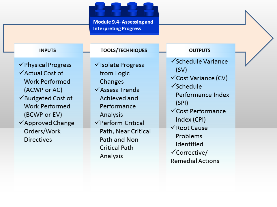
Figure 1 - The Assessing and Interpreting Progress Data Process Map

Source: Guild of Project Controls

09.4.1 INTRODUCTION

Having collected physical progress using one or more of the 11 methods described above, along with the Actual Start (AS), Actual Finish (AF) and Remaining Durations (RD) and having captured our Actual Cost of Work Performed (BCWP or AC) and having our early and late date S Curves (Performance Measurement Baselines) we are now ready to start our Earned Value Analysis and related or supporting analysis, including but not limited to confirming “as built” schedule accuracy against the baseline plan. 

In this Module 9.4 - Assessing & Interpreting Progress Data (Looking Back), we will be focusing on the progress from the beginning of the project up until the current data date or time now line and in the next Module 9.5 - Project Performance Forecasting we will be looking into the future (Forecasting).

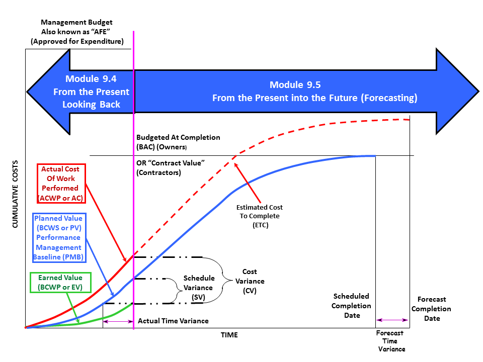
Figure 2 - S Curve Showing Focus of Module 9.4 - Assessing & Interpreting Progress & Module 9.5 - Project Performance Forecasting

Source: Adapted from DAU Gold Card KPI’s, 2015

09.4.2 INPUTS

• Physical Progress
• Budgeted Cost Of Work Performed (Bcwp Or Ev)
• Actual Cost Of Work Performed (Acwp Or Ac)
• Budgeted Cost Of Work Scheduled (Bcws Or Pv) Early And Late Date Curves
• Approved Change Orders / Work Directives & Instructions

Figure 3 - A more detailed look at the Inputs and Outputs from using Earned Value 

Source: Adapted from DAU Gold Card KPI’s, 2015

09.4.3 TOOLS & TECHNIQUES

As with all the tools and techniques shown below, there are simply too many variables to tell you which tool should be used in any given circumstance.It is up to you as a practitioner to KNOW and UNDERSTAND how to use each of these tools and techniques and in the event you are unsure which one is “better” or “best” in any given circumstance it is up to you to seek out advice from your supervisor or mentor.

09.4.3.1 Isolate Progress from Logic Changes

When an OWNER receives a schedule submitted by the CONTRACTOR (the same applies when a contractor received a schedule from a sub-contractor), there are certain “quality control” checks which need to be run.  It would also be wise for the contractor to perform the same quality tests BEFORE submitting to the owner, knowing that the owner will be running these tests.

These tests are largely identical to those performed in Module 7.7 Validate the Critical Path & Completion Dates, Module 7.8 - Validate Horizontal & Vertical Integration and Module 7.9 - Conducting a Schedule Risk Analysis, except instead of being performed on the Baseline Schedule, they are now being applied to each and every UPDATE as well.

09.4.3.1.1 Out of Sequence Progress

The first of these quality checks is to see if there is “Out of Sequence Progress”. Out of Sequence Progress is defined to be “executing work in a different order or sequence than that shown in the CPM schedule”. (e.g. In the schedule, the relationship between Activity A to Activity B was Finish to Start in the baseline schedule, but when the actual start information came in from the field it showed that in actuality, Activity A started and then 5 days later, before Activity A finished, Activity B started. Thus indicating that the logic SHOULD have been Start to Start with a 5 day lag and NOT Finish to Start as originally scheduled.

The danger of NOT fixing out of sequence progress is that in many of the more popular scheduling programs if there is out of sequence progress, any earned value for those activities which are out of sequence will be IGNORED or not credited.

To identify out of sequence progress, the more sophisticated scheduling software will produce an out of sequence progress report while other software packages, you will need to compare previous periods against current periods, inspecting the logic manually.

09.4.3.1.2 Open Ends

Open ends was explained and illustrated in Module 7.5.3.4 Incomplete and Dangling Logic.  As with Out of Sequence Progress, the more sophisticated software will generate an “open ends” report while for the less sophisticated programs, you will have to inspect each activity individually (tabular) to ensure that all activities have at least one successor and at least one predecessor, and preferably not more than 3, which should also trigger an evaluation by both the owner and contractor’s planner scheduler, as more than 3 predecessors significantly increases the riskiness of that activity starting on time.

09.4.3.1.3 Changed / Modified Logic

Whenever logic has been revised from the baseline plan the contractor, or the contractors sub-contractor / consultant should identify those changes in logic, explaining or justifying why they were made.  As a caution to project controls teams some of the less scrupulous contractors will make changes in the logic which work to their advantage.  So reviewing and challenging unexplained or unauthorized logic changes is a serious responsibility project planners / schedulers.

Initially, changes in the logic should be noted in the “NOTES” field of each activity, but then a summary of all logic changes should be included in the periodic schedule narrative report or transmittal cover letter when submitting the schedule to the relevant stakeholders.

If schedule logic is continuously revised each update period to reflect the actual sequence of work in the field significantly differing from the planned work sequence, it serves as an indication that the schedule was not developed properly indicating that a schedule review might be warranted to determine if a re-baseline or even a recovery plan is needed.

09.4.3.2 Assess Trends Achieved & Performance Analysis

09.4.3.2.1 Introducing the “S” Curve

Regardless of which software package is used, all of them use pretty much the same algorithm’s to generate the “S” curve. This example was done in Excel just to show the mechanics the scheduling software packages use. Also keep in mind that many people still do use Excel as the basis for their scheduling.

Keep in mind that the example below is the CONTRACTOR’s cost loaded schedule as submitted to the OWNER as a contractual requirement from Module 7.10 Communicating the Baseline Schedule. As such if the owner wants to use the contractors S curve as the basis for the OWNER’s performance measurement baseline, they (Owner’s Project Control Team) has to ADD additional activities to cover the Owner’s Project Management as well as other “owners project overhead” costs, such as Safety, QA/QC, owner supplied equipment or services. Depending on the policies of the owner company it may also include project finance costs.

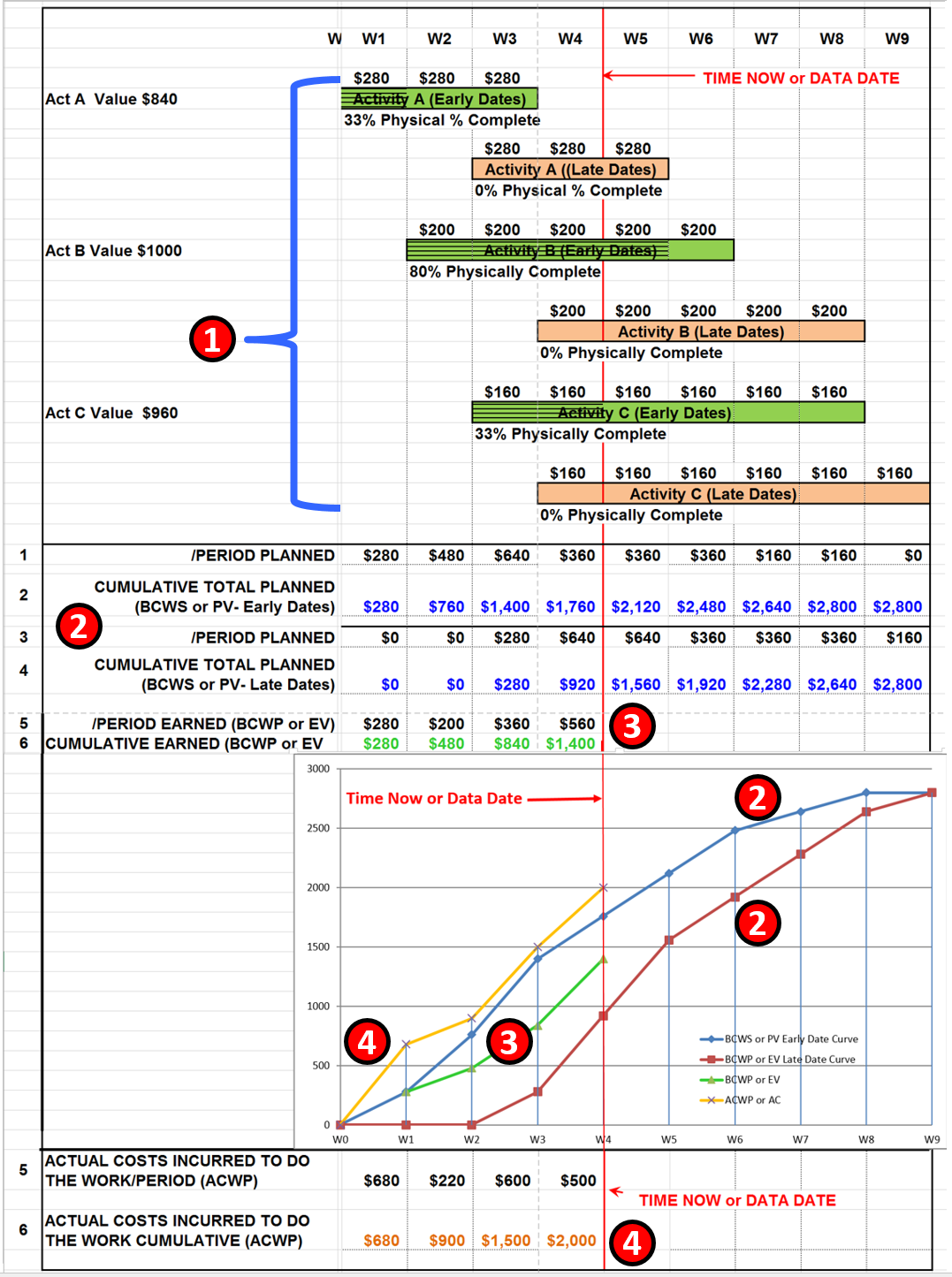
Figure 4 - How “S” Curves are Generated

Source: Giammalvo, Paul D (2015) Course Materials Contributed Under Creative Commons License BY v 4.0

In Figure 4 above, we can see:

1. Each Activity must be cost loaded including both owner and contractor activities. In the example above this schedule contains ONLY the Contractors Activities. Important to remember that the values shown here are not the contractor’s COSTS but his SELLING PRICE- meaning they are the OWNERS COSTS at the point when the work is completed and billed by the contractor and paid by the owner.
2. The project control team needs to generate both the early and late date curves using the CUMULATIVE COSTS over time.
3. Using one of the 11 methods shown in Module 09.2, we need to generate the Earned Value (BCWS or PV X Physical % Complete) per activity, add them up for each work PERIOD, then accumulate the costs over time.
4. From Module 09.3 - Capturing Progress & Updating the Schedule, we have to obtain the Actual Cost of Work Performed (ACWP or AC) from Accounting/Finance in real time or if we are not able to obtain ACWP in real time, then we need to capture it within the project controls department.  Note, this step may also be required for Contractors for any portion of the work they subcontract out, as they too may have a time lag between the time their subs/vendors do the work and when the contractor receives and is able to process the billings from those subs/vendors.

Important remember that we do NOT plot the per period values for the BCWS, BCWP or ACWP but only the CUMULATIVE values.

Important also to note that the above "S" curve example does not include the possible projections that can be made using the above basic "S" Curve data; this is covered in Module 09.5 - Project Performance Forecasting where we will be looking into the future (Forecasting).

A real life example of what Figure 4 is showing has been provided to us by Rafael Davila in a posting on the Guild Forum, dated Tue, 2016-06-07 06:26:

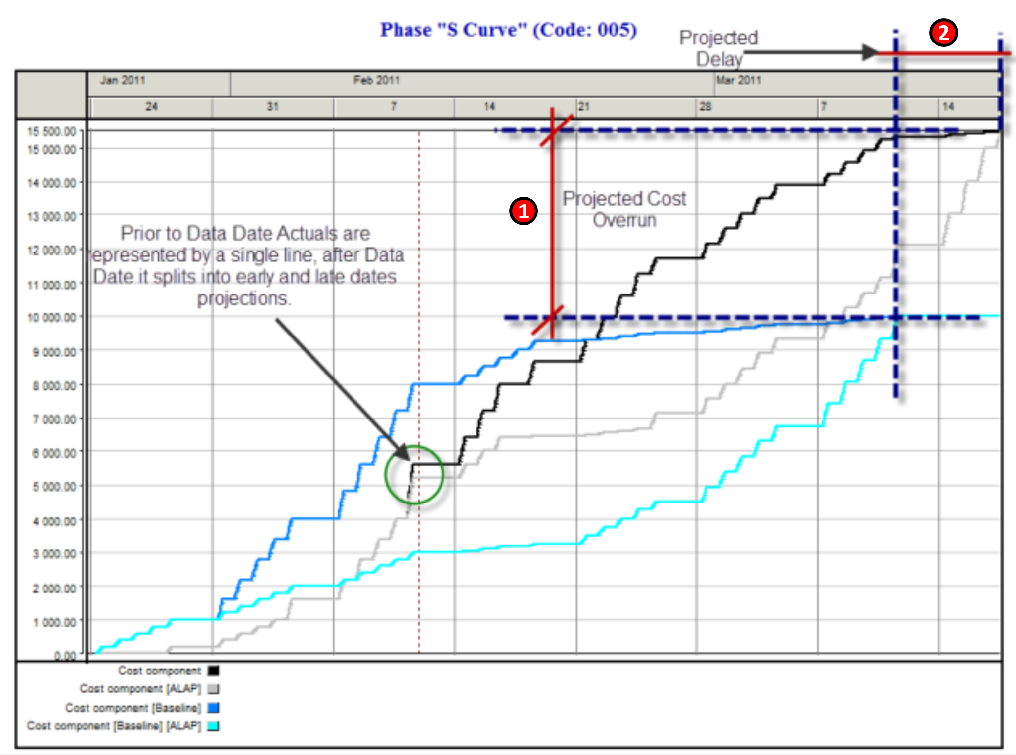
Figure 5 - Actual Example Showing the Projected Cost and Schedule Over-Runs

Source: Davila, Rafael Guild Forum, Tue, 2016-06-07 06:26

In this example, we can see how the "S" curve can assist in understanding where the current progress may take you as a result of todays progress.  From Figure 5 we can clearly see (1) the difference between the original BCWS or Planned Value (PV) and the Early and Late Date Projected Costs and (2) the Original Baseline Completion Date and the Revised or Rebaselined Completion date.  This is covered in Module 09.5 - Project Performance Forecasting where we will be looking into the future (i.e. Forecasting).

There are many different tools & technique’s we can use to measure, assess and evaluate the health of our projects using the basic principles underlying Earned Value Management but first and foremost is the Project “S” Curve, which is also known as the Performance Measurement Baseline or PMB. As many of the tools and technique’s used both to analyse the past as well as predict the future come to us from the “S” Curve, we want to start out by introducing it and explaining the components.

In the subsequent headings, we will explain how to calculate these values, why they are important and how you use them as the basis to make recommendations to the project manager or other key stakeholders.

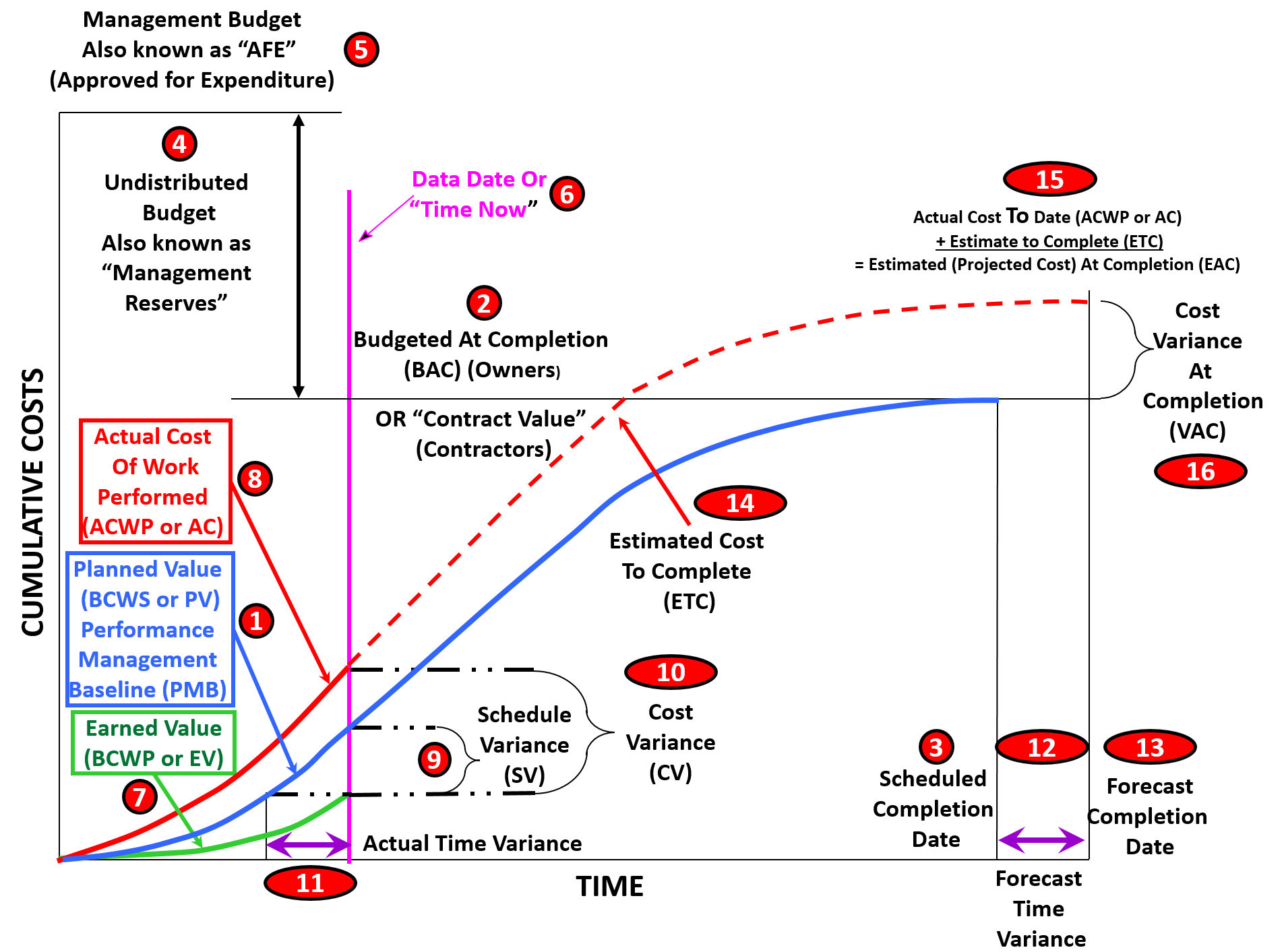
Figure 6 - Complete “S” Curve or Performance Measurement Baseline (PMB) 

Source: Adapted from DAU Gold Card KPI’s, 2015

1. Budgeted Cost of Work Scheduled (BCWS) sometimes called “Planned Value” (PV) This is generated by COST LOADING the activities in the CPM scheduling software. (See Module 07- Managing Planning and Scheduling and Module 8- Managing Cost Estimating and Budgeting for more) For CONTRACTORS it contains our SELLING PRICE to the OWNER and thus includes our direct costs, indirect costs, project overhead costs, home office overhead costs, risk contingency and our profit margin. The value of our “S” Curve should EXACTLY equal the contract value (2) on the day we commence work spread out out until the Contract Completion Date (3). For OWNERS, we need to take the cost loaded schedule submitted to us by the CONTRACTOR, and ADD to that our own project management overhead activities (e.g. Project Management, QA/QC, and Safety etc) as well as any risk or time CONTINGENCY which is owned/controlled by the project management team. As a project is not a PROFIT CENTER for an owner, there is no profit margin included in the owner’s activities. As owners, we also need to add in any Owner Supplied Equipment or Owner Supplied Materials. For owners, this is known as the “Budget At Completion” or BAC (2) and is spread out over the Contract Completion Date, which forms the Early or Target Completion Date for the Owner (3). Also be sure to note that while only the EARLY DATE BCWS or PV was shown, “best tested and proven practice” indicates that BOTH the Early Date and Late Date “S” curves should be shown.
2. Budget at Completion (BAC) is what the owner’s project control team calls their “cost loaded schedule” which because of owner’s project overheads, risk contingency, owner supplied materials or equipment, will always be larger than that of the contractor. For the contractor, this same value is known as the “Contract Value” and exactly equals the amount shown on the contract as signed. It may change but to start out, it must be exactly the same value.
3. Scheduled Completion Date- For both Contractor and Owner, this is the scheduled completion date as stated in the contract documents.
4. Management Reserves- While contractors load the activities with their SELLING PRICE, which includes the contractor’s profit margin, for owner’s UNALLOCATED money which was designed to cover “Unknown-Unknowns” is NOT included in the Owner’s Performance Measurement Baseline. The reason behind this is because “unallocated budgets” do not belong to the owner’s project manager, but to a higher level of management, which is why it is known as “Management Reserve”. If the project manager needs or wants to access this money, he/she needs to make a case for why it is needed and seek out permission to have it transferred from the “Management Reserve” account over to one or more work packages or activities on the project.
5. Approved for Expenditure (AFE)- The Owner’s Budget At Completion (BAC) plus the Management Reserve is often known as the “Approved for Expenditure” (AFE). This is the total amount upon which the business case was predicated and only under extenuating circumstances should the AFE value be exceeded.
6. “Time Now” or “Data Date”- Up to this point the information contained in Items 1-5 should have been in place BEFORE the physical execution of the project started. While this is often not the case, it is a less than desirable practice to begin work without a contract in place and a performance measurement baseline established. The Time Now or Data Date establishes the date on which the schedule was updated and analysed.
7. Budgeted Cost of Work Performed (BCWP) or Earned Value (EV)- As construction or execution of the project begins, we start to measure physical progress.  This is known as “Budgeted Cost of Work Performed” (BCWP) or “Earned Value” (EV).  As noted above, while only the Early Date BCWS was shown, “best tested and proven” practice indicates that BOTH the Early and Late Date BCWS curves should be included. Why? Because while rarely will contractors beat the early dates, what is really important is to make sure the project doesn’t breach the late date curve. Doing so is a sure indication that our project has negative float.
8. Actual Cost of Work Performed (ACWP) or “Actual Cost” (AC)- As work progresses both owner and contractor are incurring costs against that work. This is known as the Actual Cost of Work Performed (ACWP) or “Actual Cost” (AC). As we know from Module 09.3 - Capturing Progress & Updating the Schedule, the owner is unlikely to know the CONTRACTOR’s ACWP and that when the contractor bills the owner for their BCWP, the Contractors BCWP becomes the OWNER’S ACWP but, the owner also has to add in the cost of his/her project overheads, owner supplied materials and equipment. This means the OWNER’s ACWP will always be HIGHER than that of the Contractors.
9. Schedule Variance (SV) compares the amount of money EARNED vs the Amount of Money that was SCHEDULED TO BE EARNED as of the data date. As we can see from a quick visual inspection that because the amount earned is LESS than the amount of money that should have been earned by this date that the work progress is behind schedule. The formula to calculate this will be explained in more detail below as well as how to use this information.
10. Cost Variance (CV)- compares the amount of money actually spent to date against the amount of money that we planned to spend, and here again, a simple visual inspection shows us that because the Actual Cost of Work Performed (ACWP) is HIGHER than our Budgeted Cost of Work Performed (BCWP) or “Earned Value” (EV) that this project is already in deep trouble from a cost perspective.
11. Actual Amount of Time Behind Schedule- It is very difficult to talk to management in terms of how much money ahead or behind schedule we may be, so in order to communicate effectively with our stakeholders, we need to convert the Schedule Variance into days or work periods we are behind or ahead of schedule. How to do this and how to use what it tells us will be explained in more detail below.
12. Forecast Time Variance- If we take the information shown in 11 above and project if forward, it will give us a “quick and dirty” projection of when the project will finish.
13. Forecast Completion Date- If we add the Forecast Time Variance from 11 and ADD it to the current target or contractual completion date, it will give us a “quick and dirty” projection of when the project will finish.
14. Estimate to Complete (ETC)- We can use the Actual Cost of Work Performed (ACWP or AC) to date and use that information to predict into the future, what the project will cost.
15. To accomplish that, we take the Actual Cost of Work Performed (ACWP or AC) which is also known as the “sunk costs” and add to it the “Estimate to Complete” (ETC) and it will give us the projected “Estimate at Completion” in terms of money.
16. Variance at Completion (VAC) If we deduct the Baselined BAC (owners) from the most recent Estimate at Completion (EAC) it will tell us what the projected Cost Variance At Completion will be. Likewise for Contractors, we too can do the same thing. By deducting our original contract value from the latest Estimate At Completion (EAC) we too can tell if we are in trouble or not.

09.4.3.2.2 Key Elements for INTERPRETING PROGRESS DATA (from the PRESENT looking BACK)

Because there is so much to cover, the explanation of how to use and interepret the use of cost and schedule information generated using Earned Value has been broken down into two parts. In this module we will be focusing on the progress from the beginning of the project up until the current data date or time now line. 

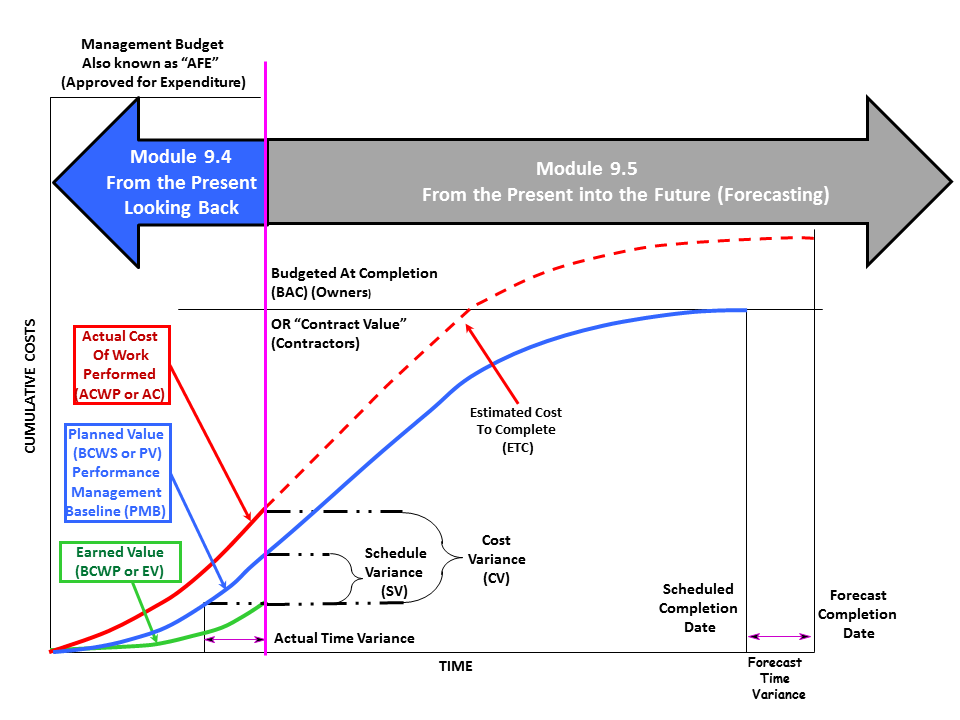
Figure 7 - S Curve Showing Focus of Module 9.4 Assessing & Interpreting Progress & Module 9.5 Project Performance Forecasting 

Source: Adapted from DAU Gold Card KPI’s, 2015

09.4.3.2.3 Budgeted Cost of Work Scheduled (BCWS or PV)

The Budgeted Cost of Work Scheduled (BCWS or for PMI followers, PV, refer Item (1) in Figure 6 Complete “S” Curve or Performance Measurement Baseline (PMB) above) is generated by “cost” loading the CPM schedule. When we say “cost” we are talking about the owners cost, not the contractors costs. The owner’s costs are the contractors selling price. For a contractor, it includes his/her project direct costs, project indirect or overhead costs, contingency, home office indirect or overhead costs and his/her profit margin. While only the early date curve is shown in this example for clarity, this is NOT a “best tested and proven” practice. To be considered a “best tested and proven” practice both the Early Date Curve and Late Date Curves should be shown.

For owners it is important to remember that you do NOT include any unallocated MANAGEMENT RESERVES in your S Curve, as those are neither owned by nor controlled by the project manager/project team. However, CONTINGENCY (risk and estimating errors) ARE included in the OWNER’S S Curves.

The formula to calculate the Budgeted Cost of Work Performed (BCWP or for PMI followers, EV) is very simply to multiply the physical percent complete using one of the 10 methods times the BCWS or PV of that activity or work package which yields the BCWP or EV for that activity or work package. We then sum up the BCWP for all activities, divide by the Budget at Completion (BAC) and that provides us with the overall Project Percent Complete.

09.4.3.2.4 Actual Cost of Work Performed (ACWP or AC)

The Actual Cost of Work Performed (ACWP) or for PMI followers, AC, refer Item (2) in Figure 6 Complete “S” Curve or Performance Measurement Baseline (PMB) above) comes to us from accounting or finance. As explained in Module 09.3- Capturing and Using Actual Cost of Work Performed, we know that there is almost always a gap between work actually being done on the project and the ability to obtain real time cost information against that work. A simple Excel based solution was provided to you in Module 9.3 to address of fix this problem.

The way we use ACWP or AC is to compare what a work package or activity actually cost against what we originally estimated it would cost, the objective being to keep the ACWP or AC at or below the amount we originally estimated.

09.4.3.2.5 Budgeted Cost of Work Performed (BCWP or EV)

The Budgeted Cost of Work Performed (BCWP or EV, refer Item (3) in Figure 6 Complete “S” Curve or Performance Measurement Baseline (PMB) above) is calculated using one of the 11 methods shown in Module 09.3 to determine physical percent complete and then multiplying that percentage times the BCWS or PV for that same work package or activity, which yields the Earned Value or BCWP or EV for that activity.

The way we use BCWP or EV is the basis to measure how much work was completed in terms of the original budget, and hopefully, when we add in the comparison with the ACWP or AC we will find out that our BCWP or EV is equal to or greater than the ACWP or AC.

Not only is this the basis for determining how much money the contractor is fairly entitled to bill the owner for at the end of each billing period, but it also enables us to measure or compare the BCWP against the ACWP and BCWP against the BCWS to determine how “healthy” our project is in terms of both time and cost.

09.4.3.2.6 Schedule Variance (SV)

The formula to calculate Schedule Variance (SV, refer Item (4) in Figure 6 Complete “S” Curve or Performance Measurement Baseline (PMB) above) is BCWP – BCWS or EV-PV. What this tells us is how much work (stated in monetary value) we are either behind schedule (negative value) or ahead of schedule (positive value) we are. (For those using this reference in preparing for the GPC exams, be careful to make sure you have the correct sign, noting that a positive value is good while a negative value is bad).

This tells us how far ahead or behind schedule we are in terms of money. This is also known as the “burn rate” as it tells us how fast (or slowly) we are consuming the budget which was allocated.

09.4.3.2.7 Cost Variance (CV)

The formula to calculate Cost Variance (CV, refer Item (5) in Figure 6 Complete “S” Curve or Performance Measurement Baseline (PMB) above) is BCWP – ACWP or EV-AC. What this tells us is how much work (stated in monetary value) we are either over budget (negative value) or under budget (positive value) we are. (For those using this reference in preparing for the GPC exams, be careful to make sure you have the correct sign, noting that a positive value is good while a negative value is bad).

The Cost Variance tells us simply whether we are over or under budget for the work which has been completed and accepted by the owner.

09.4.3.2.8 Actual Time Variance (Days Early / Late)

While Schedule Variance (SV) tells us how far behind or ahead of schedule we are in terms of MONEY, in order to translate that into TIME we need to take the point where the BCWP or EV curve intersects the Time Now or Data Date and then draw a HORIZONTAL line to where it intersects the Early and Late Date curves. This will show us how far ahead or behind schedule we are in terms of actual time, I,e, Actual Amount of Time Behind Schedule (refer Item (11) in Figure 6 Complete “S” Curve or Performance Measurement Baseline (PMB) above).

As we can see from the example above, when we draw a horizontal line from where the Earned Value line intersects the Time Now or Data Date line to the early date curve, we can see we are behind schedule against the early dates. Because we do not have a Late Date curve, we are unable to tell if we are ahead or behind schedule against the late date curve.

From a practical perspective, the late date curve is more useful to project control professionals than is the early date curve, if for no other reason than if the Earned Value (BCWP or EV) crosses the late date curve, it means we have NEGATIVE FLOAT somewhere in our schedule.

For some, particularly those from PMI, refer to this as “earned schedule” however just because the IT sector and PMI just discovered it, for those who came of age in the 1960’s and 1970’s this was always part and parcel of earned value management.

09.4.3.2.9 Schedule Performance Index (SPI)

The formula to calculate the Schedule Performance Index (SPI) is BCWP/BCWS or EV/PV for the PMI folks in the audience. The SPI is a measure of how EFFICIENTLY the project manager/project team is using the physical assets (human and equipment resources) assigned to their projects. An SPI of >1 is good (within reason) while an SPI of <1 is almost always a bad sign.

09.4.3.2.10 Cost Performance Index (CPI)

The formula to calculate the Cost Performance Index (CPI) is BCWP/ACWP or EV/AC for the PMI folks in the audience. The CPI is a measure of how EFFICIENTLY the project manager/project team is using the monetary assets (financial resources) assigned to their projects. A CPI of >1 is good (within reason) while a CPI of <1 is almost always a bad sign, unless offset by an increase in the SPI.

09.4.3.2.11 Cost / Schedule Trend Report

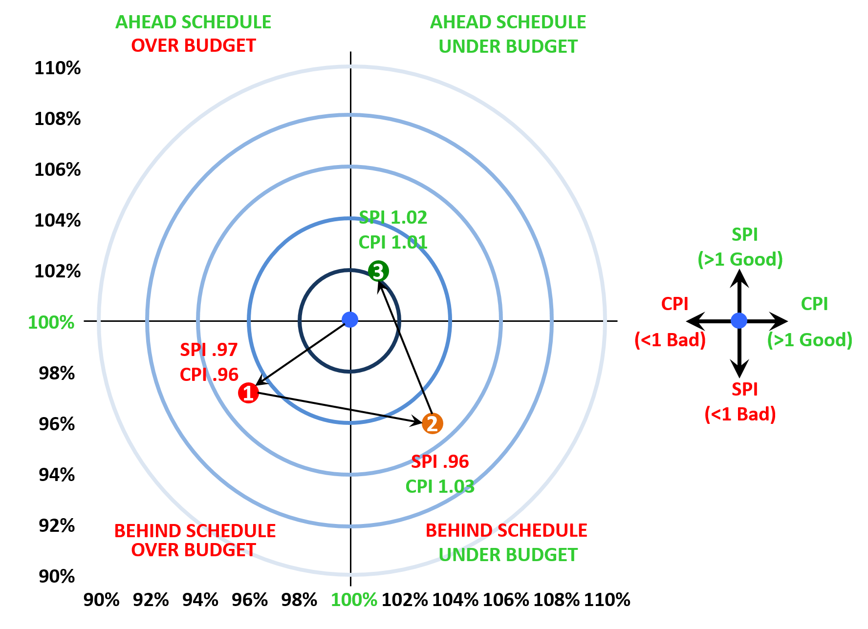
Figure 8 - Cost/Schedule Trend Report

Source: Giammalvo, Paul D (2015)   Course Materials. Contributed Under Creative Commons License BY v 4.0

In Figure 8 above, we can see how SPI and CPI can be used in a dashboard report. We plot the SPI on the vertical or X axis and the CPI on the horizontal or Y axis. The target or “bullseye” is SPI = 1 and CPI =1. These are the baseline values, and each report period we plot both the CPI and SPI, keeping in mind that the bullseye is always our target. As you can see in this example, at the end of report period 1, our SPI was 0.97 and our CIP was 0.96. This means we are 3% behind schedule and 4% over budget. Then at the end of report period 2, our SPI has gotten a little bit worse at 0.96 but now our CPI is 1.03, meaning we are now 4% behind schedule but 3% under budget. Continuing the example, at the end of report period 3, our SPI is 1.02 or 2% ahead of schedule while our CPI is 1.01 or 1% under budget.

This particular graphic is a very powerful dashboard report as it shows three items of importance to nearly all managers:

1. Are we Over Budget and Behind Schedule? Over budget but Ahead of Schedule? Behind Schedule but Under Budget? Or are we Ahead of Schedule and Under Budget?
2. Are we in trouble just a little bit (i.e. 3% or 4%) or are we in deep trouble (10% or more)

Are we getting closer to the Bullseye as this example is showing, or are we headed in a South Westerly direction? (Getting further from the Bullseye)

If you review Module 08 - Managing Cost Estimating and Budgeting that we can tell a lot about our estimates by looking at the patterns created over time by our periodic reports. Applying this same concept to SPI and CPI can provide the professional project controller with valuable information about the Accuracy, Precision and Reliability of his or her baseline cost and duration estimates.

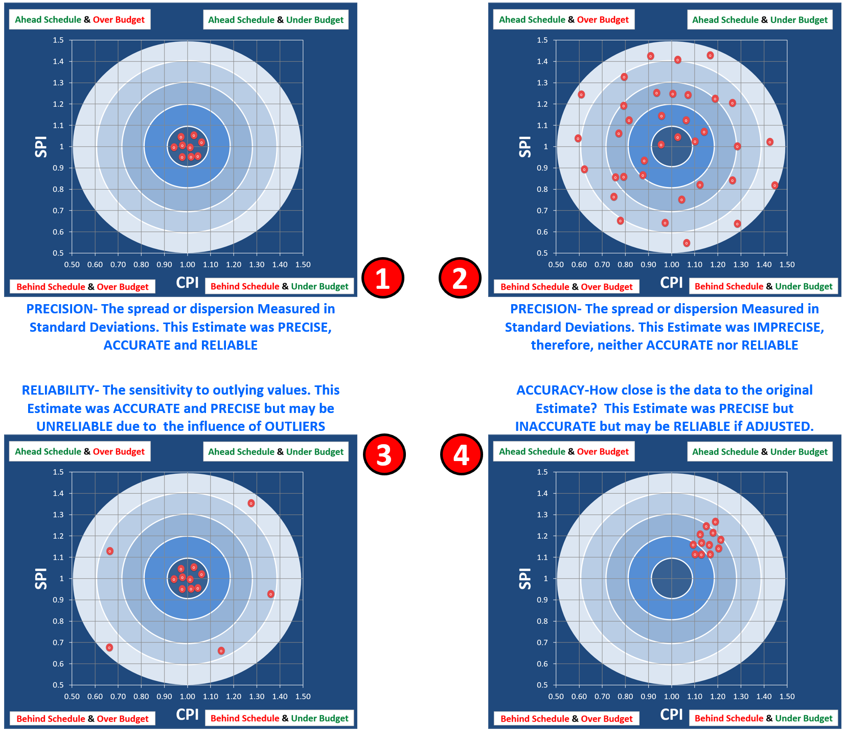
Figure 9 - Illustrating the Concepts of Precision vs Accuracy vs Reliability 

Source: Giammalvo, Paul D (2015)   Course Materials. Adapted from Adapted from Rizo, Chris (1999) “Precision, Accuracy and Reliability Illustrated and Contributed Under Creative Commons License BY v 4.0 

The 4 Scenarios explained:

1. In Scenario 1, the efficiency, as measured by the SPI and CPI are consistently falling with the acceptable target ranges. This means our original baseline estimate was PRECISE, ACCURATE and therefore, is RELIABLE to use for FUTURE PROJECTIONS in terms of both time and cost.
2. In Scenario 2, the periodic readings are all over the place. This means our baseline estimate was IMPRECISE, therefore it was neither ACCURATE nor RELIABLE to use to predict into the future.
3. In Scenario 3, while most of our periodic SPI and CPI report readings have been PRECISE, ACCURATE and therefore RELIABLE, we have to ASSESS THE IMPACT of the OUTLIERS. In this situation the project control professional could apply statistical process control chart analysis and throw out those readings which fall outside of +/- 3 sigma as being “special” or “identifiable” causes. In this scenario, using these values to predict the future without running a statistical process control check on them is risky.
4. In Scenario 4, we are getting SPI and CPI readings which are both PRECISE and RELIABLE but because they are missing the target the only way to use them would be if we adjusted the time and cost estimates to bring them back closer to the target which is one. In this particular example, because we are showing we are both ahead of schedule and under budget, we could at least CONSIDER REDUCING the remaining cost budget and SHORTENING the target completion date.

What we need to remember that the target is always 1 and that a reading which is too HIGH (>1.0) is not necessarily “good”- that overly high readings may well be a sign that the time or cost budget has been “padded” with too much contingency.

09.4.3.2.12 SPI and CPI Tracked Over Time

Another way SPI and CPI are often used is to track, compare and analyse progress over time is take the same SPI and CPI data as shown in the example above, but this time, track them per period over time (various metrics, quantities and variances van be tracked or ‘trended’ in this manner).

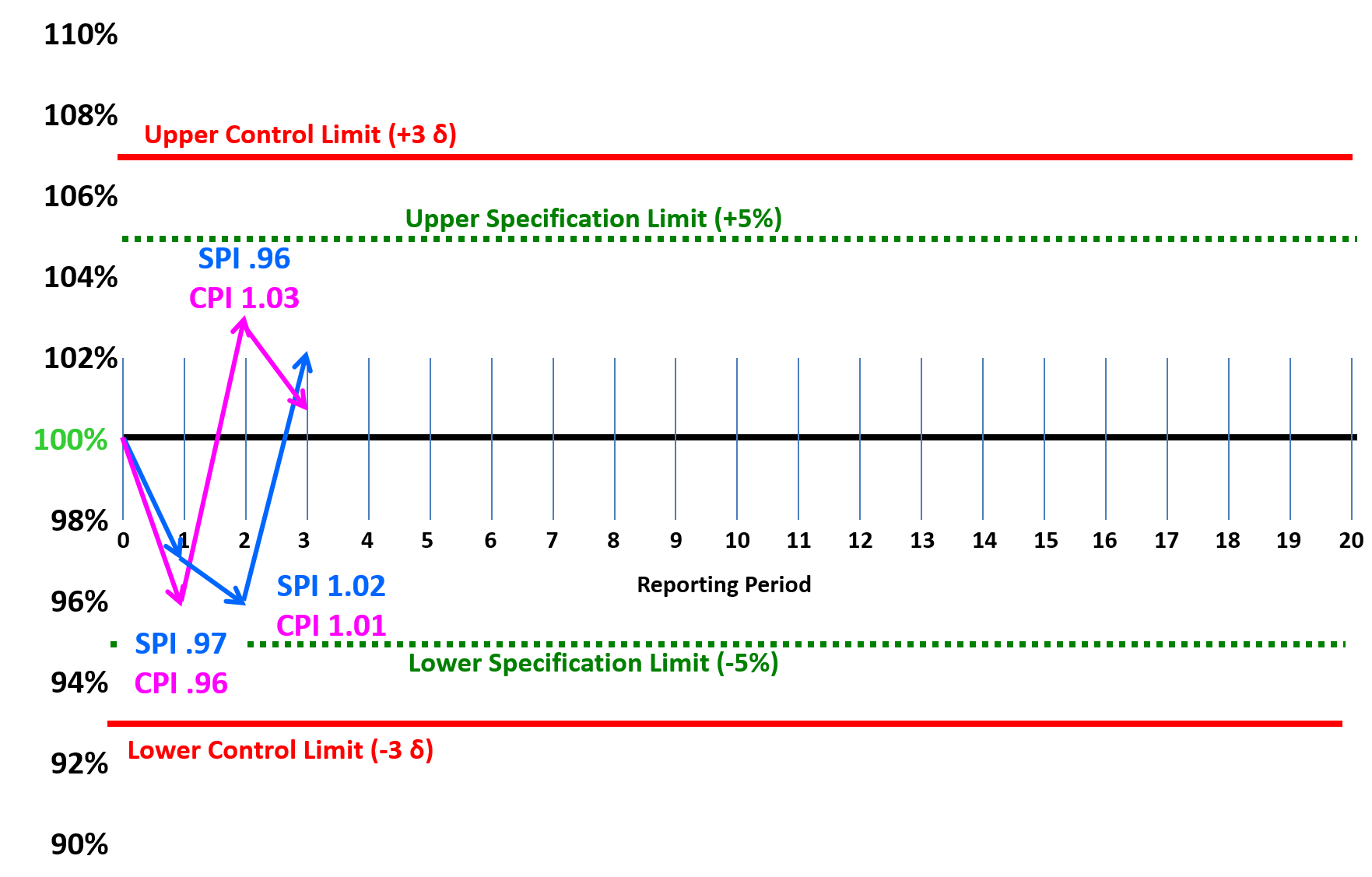
Figure 10 - SPI and CPI tracked Over Time Analysed Using Statistical Process Control Charts (SPC)

Source: Adapted from Humphrey, Gary (2011) “Project Management Using Earned Value” 2nd Edition, Figure 32-5

Depending on the audience and their sophistication in understanding Statistical Process Control Charts, this too makes a nice dashboard graphic which can be used to track, analyse and report SPI and CPI on a per Period or as a Trend basis.

Referencing the NDIA’s “Guide to Managing Programs Using Predictive Measures” (2014) we can see what their recommended ranges are for both SPI and CPI are:

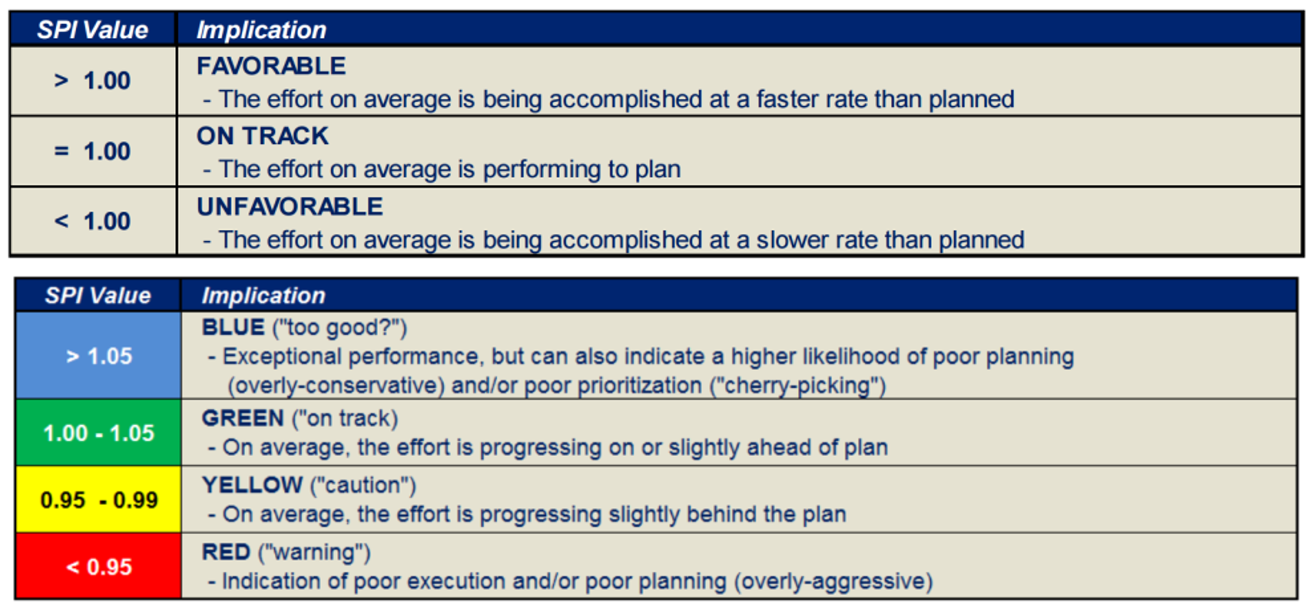
Figure 11 - SPI values from the NDIA’s Guide to Managing Programs Using Predictive Measures page 6

Source: NDIA’s “Guide to Managing Programs Using Predictive Measures” (2014)

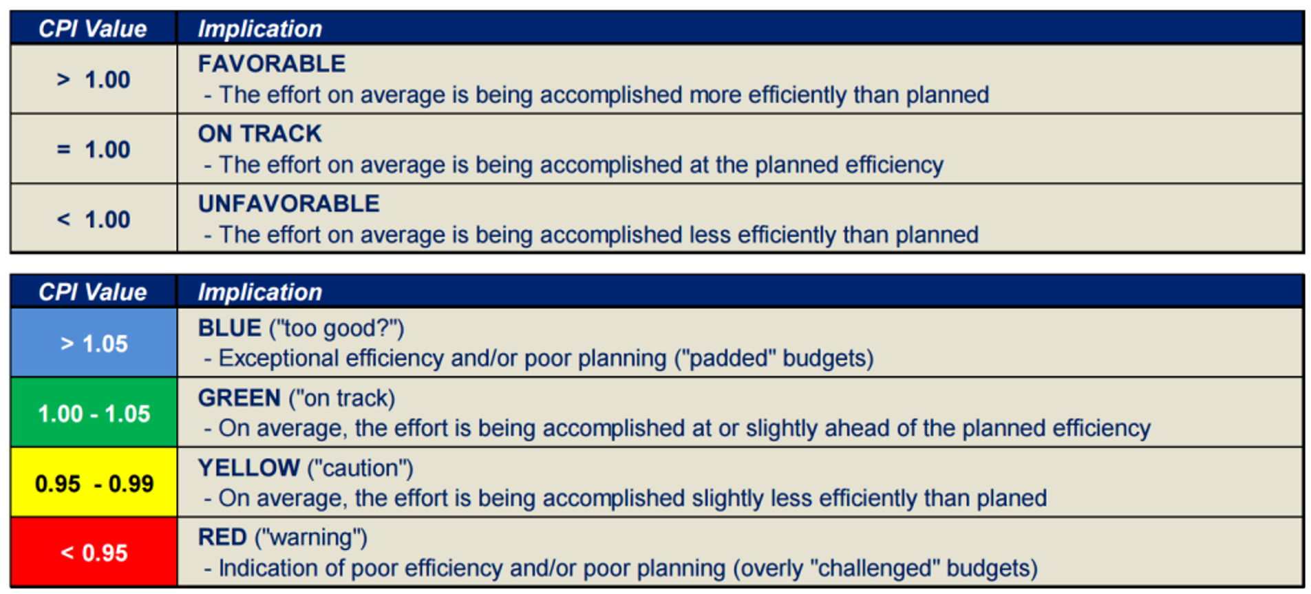
Figure 12 - CPI values from the NDIA’s Guide to Managing Programs Using Predictive Measures page 42

Source: NDIA’s “Guide to Managing Programs Using Predictive Measures” (2014)

As you can see, any readings >1.05 are considered to be “Too Good”.

For a case study showing what this means and how we can and should be using it, see below "IEAC1".

09.4.3.2.13 Baseline Execution Index (BEI) or Current Execution Index (CEI)

Another very useful metric that management likes to see is the Baseline Execution Index or BEI. There are two formulas we can use, one for starts and the other for finishes:

• BEI(Starts) = # of activities with ACTUAL starts prior to the data date/# of activities with PLANNED starts prior to the data date
• BEI(Finishes) = # of activities with ACTUAL finishes prior to the data date/# of activities with PLANNED finishes prior to the data date

The way we create the Current Execution Index (CEI) or Baseline Execution Index (BEI) is at the beginning of a report period (say a month) we count up how many activities are scheduled to finish in that time frame. Then at the end of the month, we count up how many actually did finish and it gives us a “grade” for that period. Note that this report can also show the planned vs actual STARTS as well.

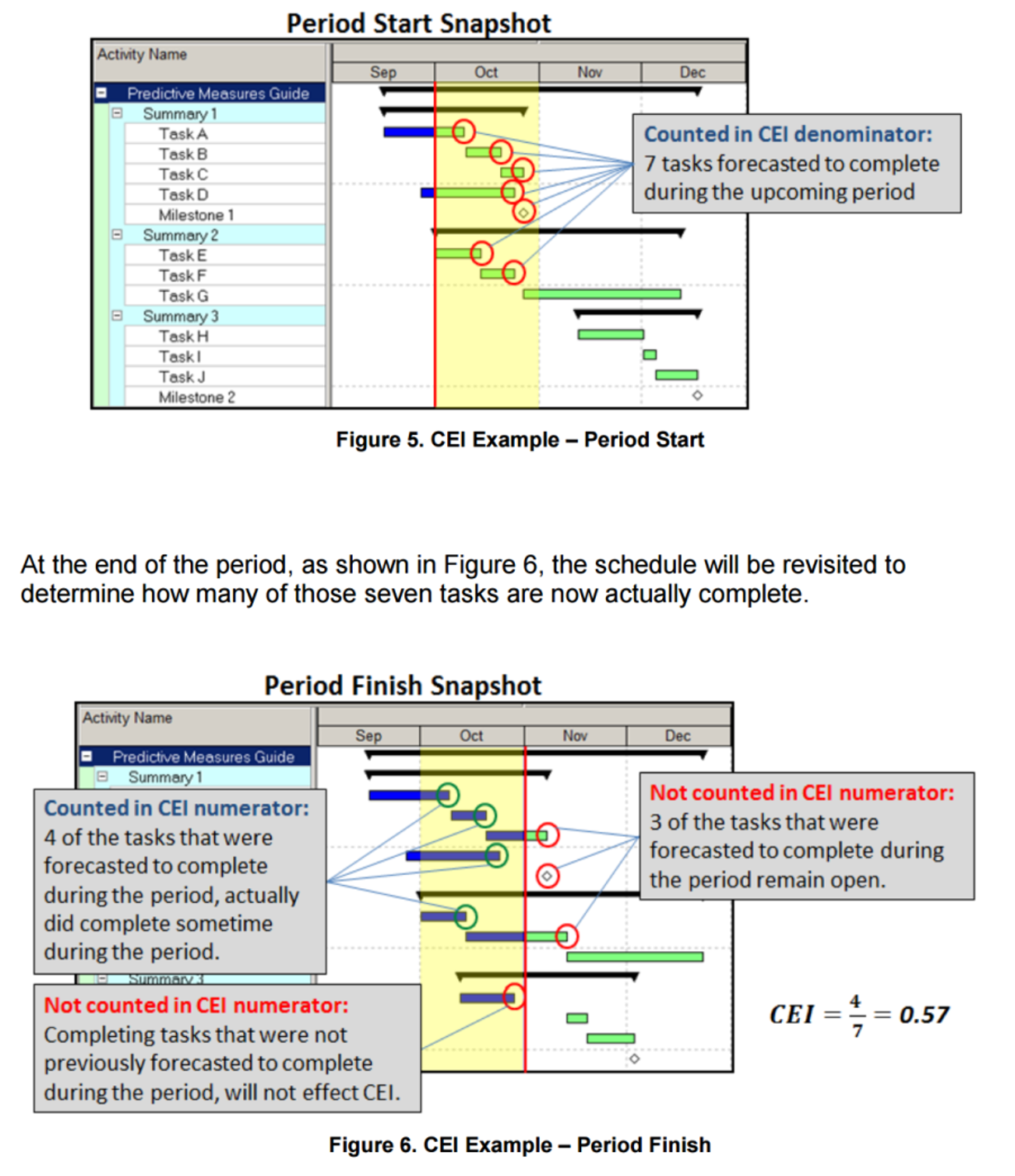
Figure 13 - NDIA Example of Current Execution Index (CEI) 

Source: NDIA’s “Guide to Managing Programs Using Predictive Measures” (2014)

Obviously enough, as with the SPI, CPI and BEI, what we want to see are values >1.0 and any score or grade <1.0 is cause for concern. Clearly from the example above, a CEI of only 0.57 stands as an early warning sign or “risk trigger” that our project is headed for trouble, and that corrective or remedial actions need to be initiated. Exactly what those might be depend on the nature of the project, but generally speaking, not starting or finishing tasks on schedule indicates either an unrealistic duration of the activities OR problems with resources. (not enough, the wrong resources or low productivity).

The action for the project control professional is to conduct a root cause analysis to found out WHY so many activities are starting or finishing late and then make recommendation(s) to improve the CEI/BEI score to as close to 1 as possible.

While a somewhat simplistic measurement (it doesn’t take into account which activities are critical or the different duration or monetary value of activities) is does provide an overall picture of how well we are doing. This KPI is comparable to batting averages in baseball or “shots on goal” (percentages of goals scored as a function of how many attempts to score were made) seen in ice hockey and soccer / football.

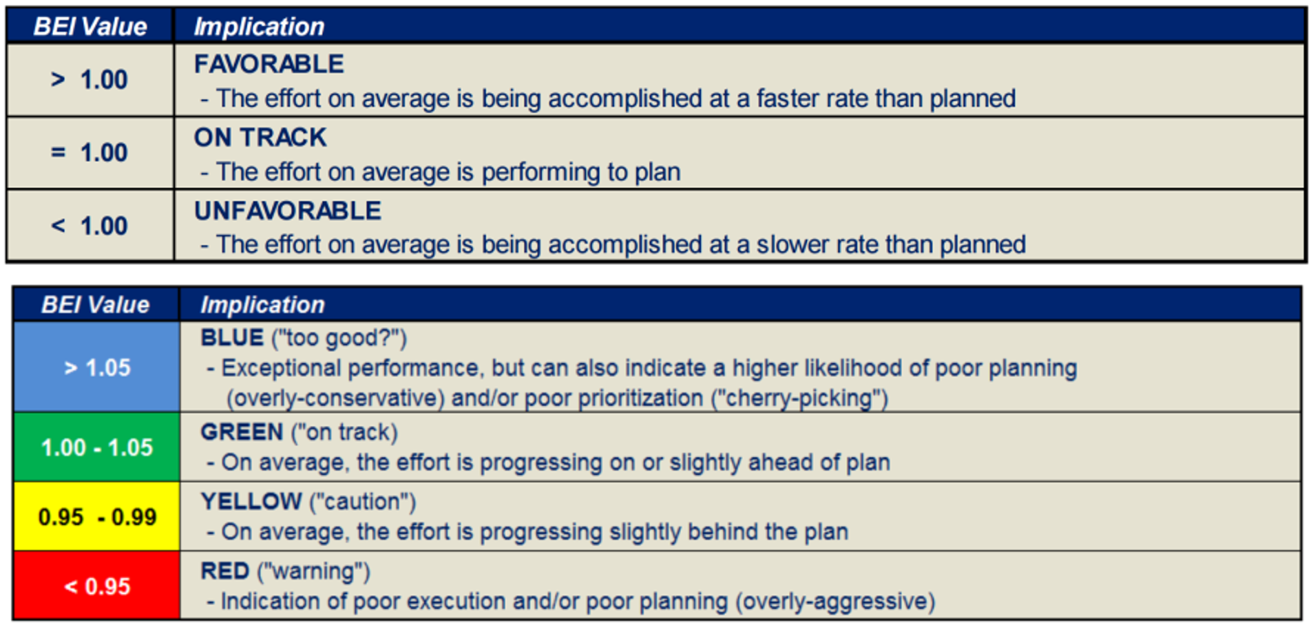
Figure 14 - BEI values from the NDIA’s Guide to Managing Programs Using Predictive Measures

Source: NDIA’s “Guide to Managing Programs Using Predictive Measures” (2014)

As this is an easy to explain metric and one which provides a reasonably accurate indication of the “health” of our project, the CEI/BEI is ideal for presentation to top management. However, it is not especially useful at the project management level as it ignores which activities are critical or near critical.

09.4.3.2.14 “Overall Project Tracking”

Another “high level” metric that we often use is comparing the % elapsed time vs the % physically completed vs the % of budget expended.

To calculate each of these bar charts: 

Figure 15 - Overall Project Tracking (right)

Source: NDIA’s “Guide to Managing Programs Using Predictive Measures” (2014)

OWNERS... 

• ACWP/BAC = % Spent to Date
• BCWP/BAC= % Earned to Date (Physical Progress)
• BCWS/BAC= % of Schedule Elapsed or Consumed

CONTRACTORS...

• ACWP/Baseline Cost Estimate = % Spent to Date
• BCWP/Contract Value = % Earned to Date (Physical Progress)
• BCWS/Contract Value = % of Schedule Elapsed or Consumed

The reason the contractor compares the ACWP against his/her baseline cost estimate is because the contract value includes the contractor’s profit margin.

To get a meaningful comparison, the contractor has to back out the profit and compare only the total costs (direct and indirect) against his/her original (contractual) cost estimate. (Not the contractors SELLING PRICE which is what he/she provides to the owner but the contractors actual COST estimate- Project Direct Costs, Project Overhead or Indirect costs.

As this is the basis to measure and analyse how the contractors project manager/construction manager is managing the money over which he/she has control over, it also does not include the contractor’s home office overhead costs, over which the project or construction manager has little if any control.)

As we can see from the example on the right, (which was taken from a real project) we can see that 87% of the time has elapsed and we’ve spent only 70% of our budget but it bought us 74% of our deliverables. Explained another way, we are 87%-74% = 13% behind schedule but we are 74%-71% = 3% under budget.

Again, hardly the kind of metrics we can use to solve day to day problems on the project but exactly the kind of “big picture” reports top management wants to see.

09.4.3.2.15 Float and Resource Analysis vs Early and Late Date Curves

Another very useful “big picture” graphic we can use to communicate quickly and clearly what our project status from the beginning to the present is to compare the current BCWP against both the early and late date curves. To create this analysis, where the BCWP curve intersected the Time Now or Data date line we draw a horizontal line which crosses both the early and late date curve.

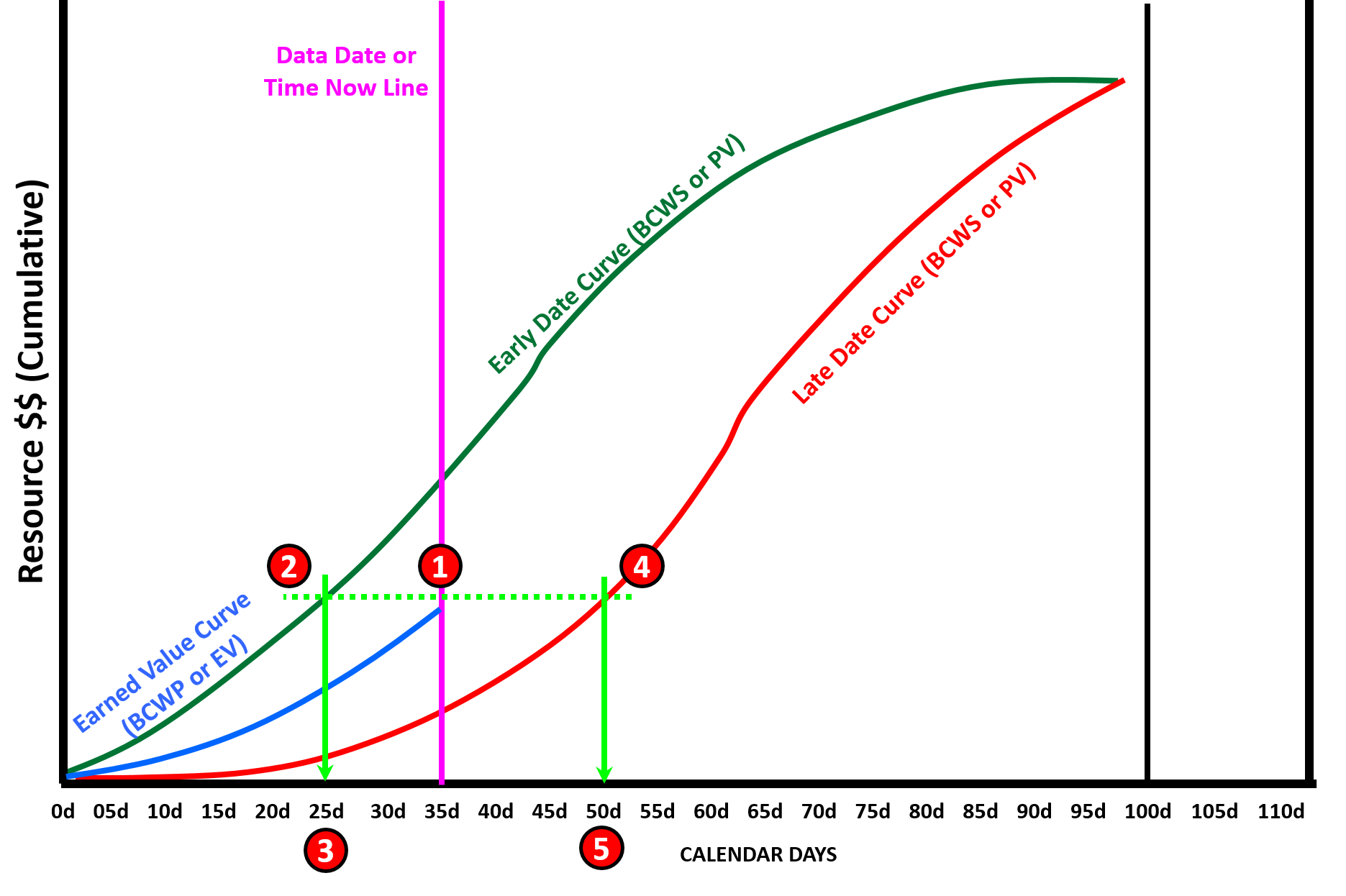
Figure 16 - Showing Both Early and Late Date Curves with the Float Analysis Illustrated

Giammalvo, Paul D (2015)  Course Materials Contributed Under Creative Commons License BY v 4.0

In Figure 16 above, we can see we have plotted both the cumulative Early and Late Date Budgeted Cost of Work Scheduled (BCWS or PV) as well as the cumulative Earned Value (BCWP or EV) curves. As we can see from the Data Date, we are now at day 35 of a 100 day schedule.

Here is the step by step process to analyse the float against both the early and late date curves:

1. Draw a HORIZONTAL LINE from where the BCWP or EV curve intersects the TIME NOW line and extend that line until it crosses both the Early and Late Date curves.
2. Drop a vertical line from where the horizontal line intersects the BCWS Early curve and we see that it indicates Day 25.
3. What this means is IF we were on schedule per the early dates, we should have been where we are today in terms of physical progress back on day 25. If we deduct 25-35 = -10 days it means we are 10 days LATE against the early date curve.
4. As we did above, we drop a vertical line from where the horizontal line intersects the BCWS late curve and we see that it indicates Day 50.
5. If we deduct 50 -35 = + 15 days meaning we are 15 days AHEAD of the late date curve, or explained another way, overall (at the project level) we have 15 days of total float before we are in danger of crossing the late date curve.

As this is a “big picture” communications graphic, as long as the contractor remains within the boundaries established by the early and late date curves, he should be in good shape. What we as project control professionals want to watch for is when the contractor’s earned value starts to approach the late date curve. This is one of the “early warning signs” or “risk triggers” we talked about in Module 3- Managing Risk that alerts us that the project, while not in trouble yet, is getting close.

Also important to note that because this is a “big picture” report, while the project as a whole may appear to have total float, we still need to check the critical path to see if this holds true at the activity level.

This is why it is so important that project control professionals get in the habit of showing BOTH the early and late date curves. Not only does this give us a “big picture” view of how much total float the project has, but also gives us an indication of how much RESOURCE FLOAT or RESOURCE FLEXIBIILITY we have.

We covered this in Module 8- Cost Loading the CPM Schedule but it is worth reiterating again here. For those of you using this publication as the basis to prepare for your GPC certification exams, as this topic is so important, you are almost sure to see questions covering this topic on your exams, especially for the Planning & Scheduling, Cost Management and Project Controls Track. Even the Forensic Analysis Track could have one or two questions on this topic.

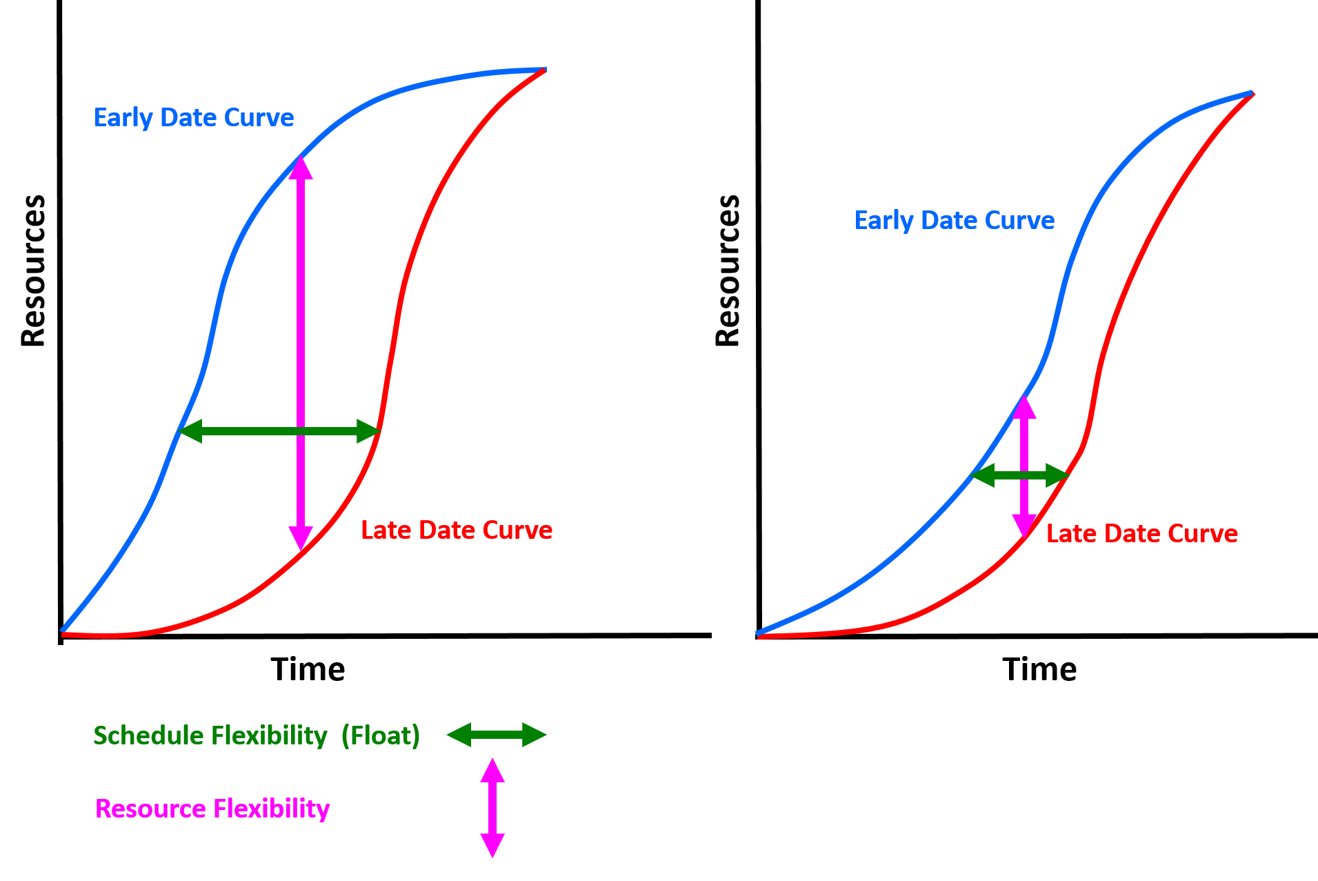
Figure 17 - Illustrating how the Early and Late Date Curves provide Resource Float and Total Float Indicators

Source: Adapted from Humphrey, Gary (2011) “Project Management Using Earned Value” 2nd Edition page, Figure 9-8

To recap from Module 8, we can see how the closer the early and late date curves are to one another horizontally, the less total float we have and thus the riskier the project schedule is. At the same time, by seeing how close together the early and late date curves are between any two points vertically, provides us with a sense of how much resource float we have, meaning how flexible we are in being able to move resources around on the project.

As explained previously, while these are “big picture” indicators of physical progress against the plan,, the project control professional still needs to check the critical and near critical path activities to see if what these summary gauges for our dashboard show are valid or not and be prepared to explain what these common dashboard gauges indicate and what they can and cannot be used for.

09.4.3.2.16 Window of Opportunity to Effect Change

One final item of importance before we get into the details of how to set up and use these S Curves - credible research by the US Dept of Defense as well as other researchers (Ibbs et al) indicate that we have a “window of opportunity” of 20% to 35% of the projects Elapsed Time in order to:

1. Identify if our project is in trouble (Yes or No)
2. If yes, identify the “root cause” problems explaining why it is in trouble and;
3. Implement corrective actions to those problems

If we fail to answer these three questions within the 20% to 35% elapsed time “Window of Opportunity”, then our projects will NEVER be able to recover.

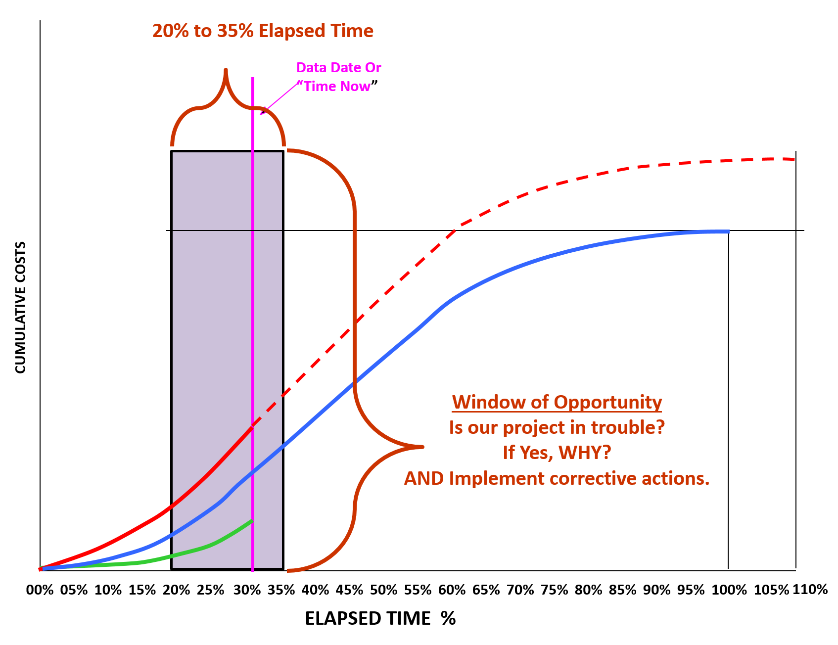
Figure 18 - Window of Opportunity to Identify Problems and Initiate Corrective Action

Source: Giammalvo, Paul D (2015) Course Materials. Contributed Under Creative Commons License BY v 4.0

This is an issue that the professional project controller needs to know and understand as not everyone is aware of this research (GAO Best Practices in Capital Budgeting Chapter 18).

09.4.3.3 Perform Critical Path, Near-Critical Path & Non-Critical Path Analysis

When comparing period to period or project start to the current period analysis, both owner’s and contractor’s planner/schedulers need to review the critical path in the current schedule compared against the baseline. The easiest way to do this is to sort (filter) only those activities which were critical in the baseline and compare it against those activities in the current report period. From this you can determine:

We also need to analyse “near critical” and “non-critical” activities. A “near critical activity” is one which has float but could possibly become critical between now and the next report period. For example if you are reporting weekly and you are working a 5 day work week, then you would consider all activities with less than or equal to 5 days float to be “near critical” as it is mathematically possible for them to go critical by the time the next report is issued. Likewise if you are reporting monthly, and you are working a 5 day work week, your definition of “near critical” would be 5 day work week X 4.3 weeks per month = 22 days. 

1. Are there any critical path activities which have slipped against the baseline?
2. Are there any NEW activities which are critical now that were not critical in the baseline?
3. Are any activities which were critical in the baseline which are no longer critical?
4. Is there more than one and/or a new critical path?

But float alone is not the ONLY determinant we need to look at. When the activity is scheduled to start is also important. Applying “common sense” an activity which has 0 total float but is scheduled to start tomorrow is certainly a higher priority than an activity with 0 float which isn’t scheduled to start until next month. While both remain on the critical path, the activity scheduled to start tomorrow has more IMPORTANT than does the one scheduled to start next month.

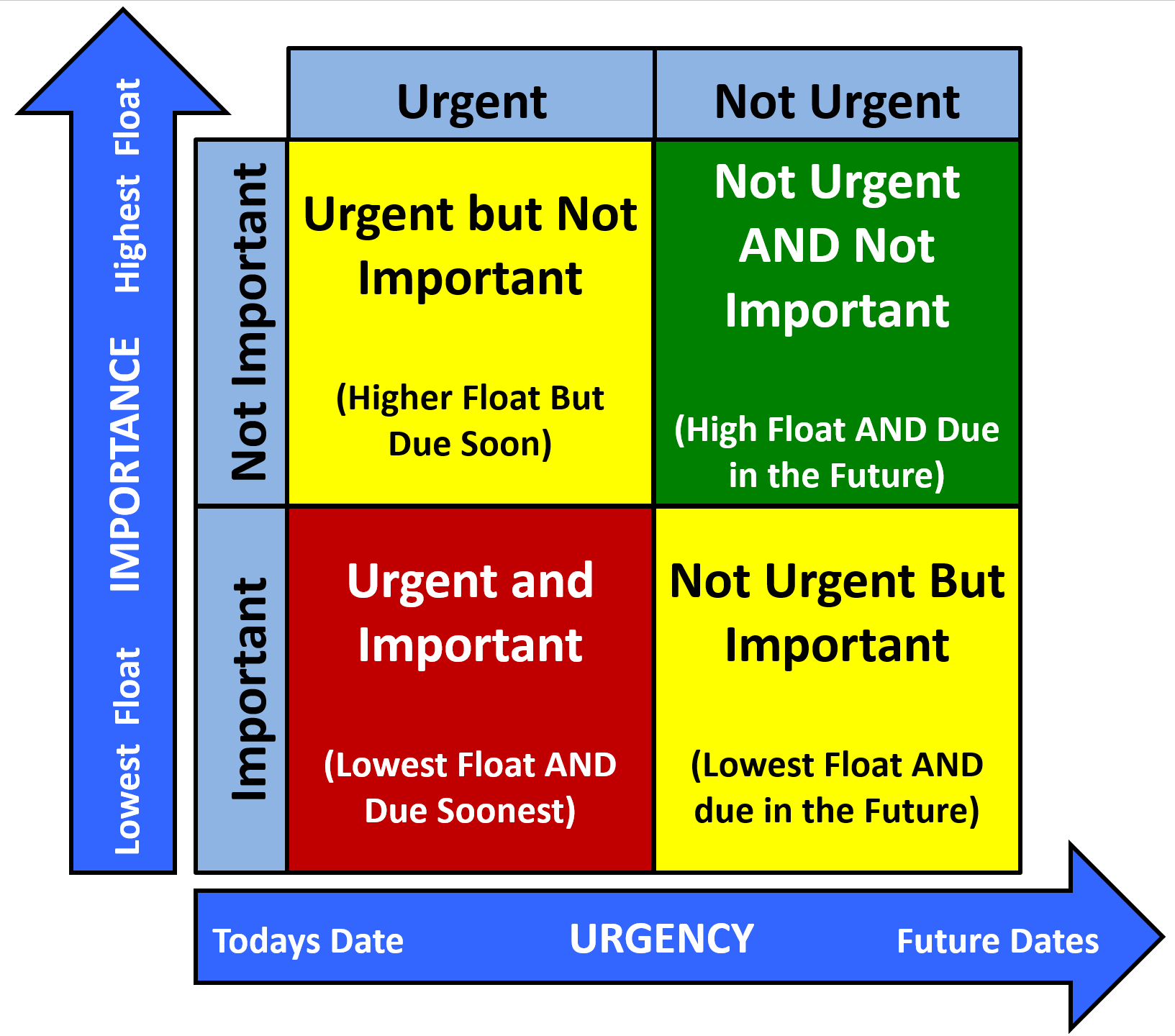
Figure 19 - Urgency vs. Importance Matrix

Source: Giammalvo, Paul D (2015) Course Materials. Adapted from Stephen Covey's Urgency vs Importance Matrix. Contributed Under Creative Commons License BY v 4.0

Figure 19 above the right which is an adaptation of Stephen Covey’s Urgency vs Importance matrix illustrates how we can and should be using both TOTAL FLOAT and SCHEDULED START DATES together as the basis to prioritize which activities require more intense management and scrutiny, both by the contractor and owner.

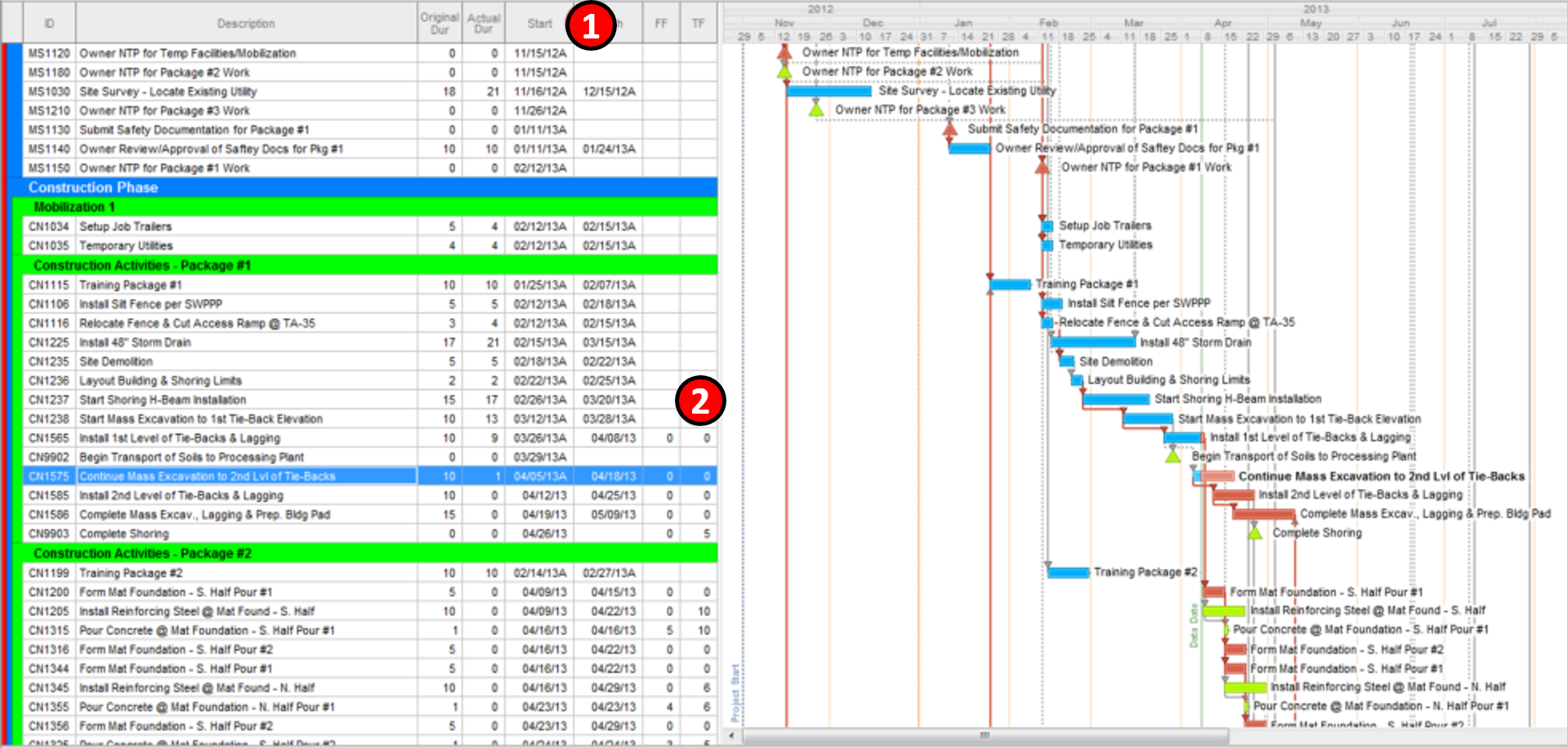
Figure 20 - Classic Schedule Sort by Early Start and Total Float 

Source: Preferred Construction Management 2015

To generate this graphic for analysis and comparison, we create a two-step sort- First sort is by Early Start Date (1) and the secondary sort is by Total Float. (2) This produces the classic “waterfall” of activities as shown above. Then we compare the Baseline against the Current Status Update, which is normally done using a bar chart format. (no logic, only a bar for the Baseline activities and a bar for the Current Activities).   See  Figure 21 below for an example of this analysis.

Using FLOAT ONLY (without looking to see when the activities are scheduled to star) the priorities are:

1. Negative Float Values (-float or Super- or Hyper- Critical activities)
2. Zero Float Values (Critical activities)
3. Float values < reporting period. (“Near Critical” activities)
4. Float values > reporting period. (“Non-Critical” activities)

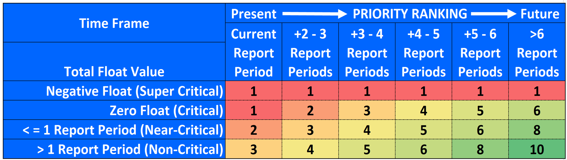
Figure 21 - Illustrating the concept of Total Float vs Time Now and Future Time

Source: Giammalvo, Paul D (2015) Course Materials Contributed Under Creative Commons License BY v 4.0

In the illustration above, using a scale of 1 (most critical) to 10 (least critical) we are trying to demonstrate the RELATIVE importance of using total float vs time now vs future time as the basis to prioritize which activities you should be focusing on, either as an owner or a contractor.

The reason we use report periods as the guideline is because it provides a handy way to scale up or down to fit any situation. While most reporting is done monthly, with tracking done weekly and data collection done daily, this same “rule of thumb” also works just as well for shut downs and turn around (scheduled or emergency maintenance on working facilities) where the reporting is done daily or even per shift, the tracking is done hourly and the data collection is done every 15 to 30 minutes. Likewise, this rule of thumb also works for high level management reporting, where we are reporting quarterly, tracking monthly and capturing data on a weekly basis. This need to be able to “roll up” and “roll down” schedules for reporting purposes is why Module 07-9- Validating Horizontal and Vertical Traceability becomes so critical, especially for owner’s project control teams.

This concept of prioritization by both total float and early start is also consistent with “Rolling Wave Planning”

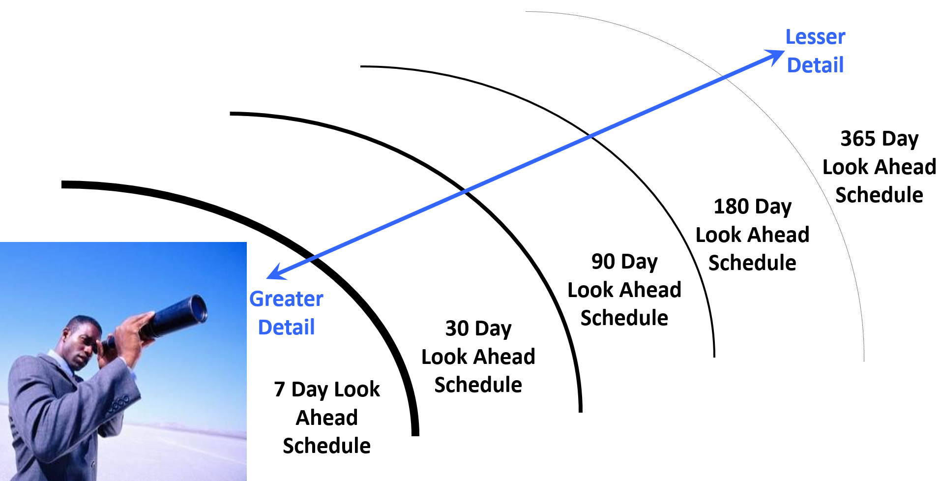
Figure 22 - “Rolling Wave Planning” Illustrated

Source: Giammalvo, Paul D (2015) Course Materials Contributed Under Creative Commons License BY v 4.0

Keep in mind these are guidelines or “rules of thumb” and it is expected that sound professional judgement will be applied as there are and always will be, exceptions to these rules.

While we can and should be sorting both the Baseline and Current Update by Early Start and Total Float, there are other sorts we can and should be looking at as the basis to compare the baseline against the current performance. This could include specific crews or subcontractors, geographic location, phases, engineering vs procurement vs construction or any other sort which provides meaningful and useful information enabling the relevant managers to make decisions based on as close to real time status of the project as is humanly possible.

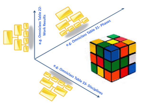
Figure 23 - Multi-Dimensional Coding Structures

Source: Moine, Jean Yves, Leynaud, Xavier and Giammalvo, PD (2015) Creating and Using Multi-Dimensional WBS Structures

As an owner’s project Control Team, having completed our analysis of Schedule Update submitted by the contractor, reviewing and analysing the critical path and having validated that the critical path contains no errors, omissions or anomalies (or that the contractor has explained and justified them) we now turn our attention to the various Earned Value analysis, which now use money as the basis against which to assess the “health” of our project in terms of both time and money.

09.4.4 OUTPUTS

• Current And Past Period Performance Metrics Calculated, Compared, Analyzed And Reported:
  • Schedule Variance (Sv)
  • Cost Variance (Cv)
  • Schedule Performance Index (Spi)
  • Cost Performance Index (Cpi)
• Root Cause Problems Identified
• Corrective/ Remedial Actions

09.4.5 REFERENCES & TEMPLATES

• GAO’s Best Practices in Capital Budgeting, Chapter 18 http://www.gao.gov/new.items/d093sp.pdf
• GAO’s Best Practices in Scheduling, Best Practice #9 pages 134-135 http://www.gao.gov/assets/600/591240.pdf
• GAO’s Best Practices in Capital Budgeting, Chapter 19, pages 270-271 http://www.gao.gov/new.items/d093sp.pdf
• GAO’s Best Practices in Scheduling, Best Practice #10 pages 150-151 http://www.gao.gov/assets/600/591240.pdf

09.5 - Module 09-5 - Project Performance Forecasting

GPCCAR M09-4 Managing Project Progress, Assessing & Interpreting Data, Revision 1.04

Revision History:

• Rev 1.01 1.03 – minor narrative improvements
• Rev 1.04 – amended error in bullet 7 and bullet 10 under Figure 6 from “Budgeted Cost of Work Performe (BCWS)" to "Budgeted Cost of Work Performed (BCWP)"