M07-10 Conducting a Schedule Risk Analysis

07.0 - MANAGING PLANNNING & SCHEDULING

07.1 - Module 07-1 - Introduction to Managing Planning & Scheduling

07.2 - Module 07-2 - Develop the Planning & Scheduling Policies & Procedures Manual

07.3 - Module 07-3 - Identify / Capture all Schedule Activities

07.4 - Module 07-4 - Create the Logical Relationships & Sequence Activities

07.5 - Module 07-5 - Assigning Resources to all Activities

07.6 - Module 07-6 - Calculate the Duration of Each Activity

07.7 - Module 07-7 - Calculating Float and the Critical Path

07.8 - Module 07-8 - Validate the Critical Path and Completion Dates

07.9 - Module 07-9 - Validate Horizontal and Vertical Integration

07.10 - MODULE 07-10 - CONDUCTING A SCHEDULE RISK ANALYSIS

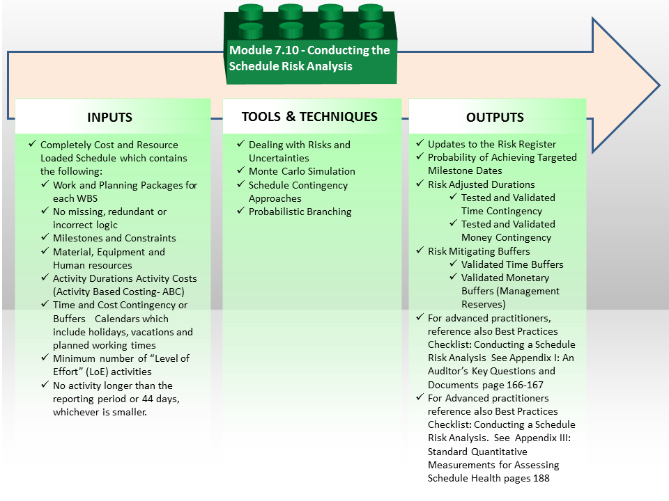
Figure 1 - Conducting a Schedule Risk Analysis Process Map

Source: Guild of Project Controls

07.10.1 INTRODUCTION

This is the third and final “quality control check” on the cost and resource loaded schedule before we officially submit it for acceptance as the performance measurement baseline. This is the final check to see if the dates targeted by management internally or through the contract documents are achievable and to what degree (percentage) probability any given date has of being achieved, be it the overall project completion or any interim milestone date.

There are differing schools of thought on whether the project should be simulated WITHOUT contingency or buffers added at the activity level and they should be added AFTER the simulation is done. On the other hand, there is a strong argument that the schedule should be simulated as “designed by the people who are going to be doing the work” which means the schedule should be simulated exactly as those executing the plan have indicated.

It is the Guild’s position that lacking any compelling reason to do otherwise, that the schedule which is going to be used as the performance measurement baseline (PMB) against which to track progress, should be simulated exactly as it was designed and agreed to by those executing the work. This means contingency and buffers at whatever level are included in the simulation model.

Worth noting is the reason that simulation is the final of the three quality control checks is because if there are any errors in logic, duration or resource allocations AND/OR if the coding structures are not complete allowing for role up/roll down, then running the simulation will be less useful and in fact may produce totally invalid results.

• The "GIGO Principle: at work- Garbage In / Garbage Out.

07.10.2 INPUTS

Completely cost and resource loaded schedule which contains the following:

• Work and planning packages for each WBS element (100% of necessary activities)
• No missing, redundant or incorrect logic
• Milestones and constraints
• Material, equipment and labourresources
• Activity durations which are realistic and achievable
• Activity costs (activity based costing- ABC)
• Time and cost contingency or buffers appropriate to the riskiness of the project, work package and/or activity
• Calendars which include holidays, vacations and planned working timesminimum number of “level of effort” (LOE)  activities
• No activity longer than the reporting period or 44 days, whichever is smaller unless otherwise justified

07.10.3 TOOLS & TECHNIQUES

07.10.3.1 Dealing with Risks and Uncertainties

Experience in project scheduling shows that the probability of successful implementation of project schedules and budgets exactly to plan can be low. This risk is mitigated by well-designed and managed project controls processes, but the initial plan can carry a large risk of failure. A Risk Management Plan is often conceived and implemented to reduce this risk of failure.

As a result of uncertainty about the modelling of the means and methods, the estimate of project completion is just that, an estimate. It will be valid only to the extent that all the estimates of task or activity durations, assumptions about sequencing and resource availability, and production rates and project conditions all turn out to be true. The quality of the model has a strong effect on the likelihood of project success, however, even with the best models, there are multiple risks to anticipate and attempt to plan. The project completed is likely not to be as projected by the schedule (or put another way; by the deterministic CPM schedule) but is likely to be somewhere in a range of dates that like any random sampling, will be spread symmetrically around that estimated completion date.

Therefore project scheduling technology benefit from the inclusion of a risk simulation to produce probabilistic modelling of the projected probable completion dates. If these dates prove to be unacceptable then the schedule development process has to loop back to the beginning and a review done of the scope, the means and methods, the logic and the durations to see if the model as simulated can be done in the allotted time and if so, what is the probability of that happening.

Although this is clearly NOT a “best tested and proven” practice, the typical CPM schedule development often does not include risk assessments, but rather is developed as if all the components of the schedule, such as duration, are exact values, known by the planner. This is one of the reasons why so many projects are finishing late, and is a major ethical issue that the professional project control professional needs to face up to and work to change.These schedules include activity durations established by calculation of the quantity of work represented by an activity divided by the assumed or historical production rate. Risk management recognizes the uncertainty in planning and provides a system to brainstorm other risks that may occur during the project.

This brainstorming essentially identifies potential risks which are stored and managed during the life of the project within a Risk Register. (See Module 4 - Managing Risk & Opportunity for an example of a Risk Register).

07.10.3.2 Duration Risk & Uncertainty

General duration uncertainty is the risk resulting from estimated durations (or costs as the two are correlated) being inaccurate or overly optimistic, based on assumptions not necessarily correct or accurate or based on the failure to conduct an adequate risk assessment.

When discussing duration uncertainty, many planners and schedulers or project members believe that their initial estimations of durations are accurate, and if the risk discussion continues, believe that their durations are the “most likely” durations. A problem with using such a “deterministic” approach is that many assumptions are made in early development of the schedule but rarely if ever questioned or reviewed again during the project.

So a “probabilistic” approach takes the concept of estimating durations based on average production rates to the next level; it looks at the range of possible project durations based on a spread (called “distribution” in statistics) in the estimated activity durations, commonly called three-point estimates of duration; the pessimistic, the most likely, and the optimistic.

The estimated durations, whether single estimates or three-point estimates, should be calculated by accurate quantities and appropriate production rates. This allows for a compiling of all general risks to the duration into this three point estimate by providing a range of durations that can be used in the risk analysis.

However, as we know from Module 4 - Managing Risk & Opportunity using the “Average” or P50 value means that 50% of the time our activity will take longer than the duration entered and 50% of the time the activity will take less time. Assuming that the two will cancel one another out is a false assumption, evidenced by the number of projects which finish late.

This means that to be a responsible professional we need to increase the probability of finishing on time, which means we cannot use the “average” or P50 value but built in a time or money contingency to raise the probability from 50% to whatever probability or comfort level management wants. Usually for an owner organization this is P85% or P90% and for a contractor, that is normally P60% to P75%.

07.10.3.3 Monte Carlo Simulation

Using such a range of durations, the Monte Carlo technique makes the analysis of duration uncertainty and activity relationships risks possible. Monte Carlo analysis runs a large number of iterations based on the spread of the three duration estimates, so that many combinations of durations are used.

This probabilistic approach recognizes that the more accurate way to model uncertainty in durations is through the use of statistics, where if enough iterations are run, the results will generally fall into one of the common probability distributions of activity durations. One of those probability distributions that is commonly seen and used is the “normal distribution”, which graphs into a bell curve with the most likely duration at the highest peak of the curve and smaller probabilities as the curve diminishes in both directions.

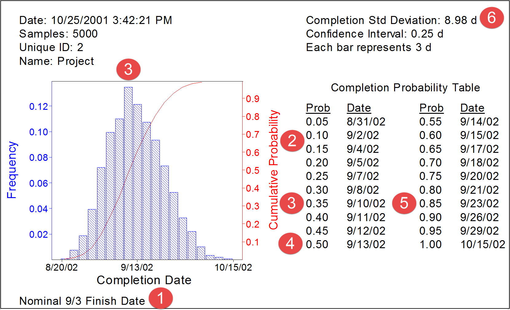
Figure 2 - Example of Output from a Monte Carlo Simulation

Source Courtesy of Hullett, David (2002)

 In the example above, a simple project schedule was simulated.

1. The target finish date established by management was 3 September
2. The probability of finishing on/before that date is about 13%
3. The “Most Likely” date of finishing is around 10 September which as a “probability” (P) of about 35% (P35)
4. The probability of finishing on or before 13 September is 50% (P50) which means that the project has a 50% chance (P50) of finishing later. This is the DANGER of using “average” or “mean” durations in our schedules.
5. The P85 (85% probability) of finishing on or before would be on 23 September.

For those familiar with statistical analysis (See Module 4 - Managing Risk & Opportunity) the Standard Deviation or Sigma (δ) is 8.98 or 9 days. This is the whole purpose of testing the “as planned” schedule one last time before formally issuing it as a baseline schedule. IF we as project control professionals were to do this AND we were able to make a compelling example to the key decision makers as to why their project completion dates were unrealistic and assuming we can convince them to listen and heed our advice, then not only would more projects finish on time but there would a lot fewer claims and disputes on projects than we currently have.

The Monte Carlo analyses provide statistically significant “confidence levels" for the probabilistic prediction of achieving specific or targeted completion dates and - since schedules are dealing with unknowns - enable the schedules to have higher probabilities of meeting the chosen completion date. One weakness with Monte Carlo simulation is that it doesn’t take into account good project controls, where analysis and feedback from periodic updates is used to modify the plan. With the use of good project controls, it is much less likely that the stacking of pessimistic durations as happens in the simulations would go unnoticed and unmitigated. However, Monte Carlo simulation provides a number of very useful metrics as well as producing comparative evaluations of completion probability.

The Monte Carlo methods are available in numerous computerised software packages which can be linked to the scheduling software or are built into the software.

In addition, the level of detail in the schedule is an important requirement for use with risk analysis. There must be enough detail to isolate each activity by responsibility. This means that, for a schedule to be used in risk analysis, an activity should only model one discipline or party. This allows evaluation of each discipline or party for different assumptions of risk, as well as evaluation of areas for different risks. This is good scheduling or programming practice in any event, so it is in the best interests of the project for the schedule to contain this level of detail.

The use of constraints can affect the validity and accuracy of risk calculations because constraints may sequester float or prevent the network from calculating correctly. It may be necessary in the risk analysis to remove constraints in order to see the impact of those constraints on project completion. In addition, the use of mandatory constraints that do not allow the network to calculate float accurately in delay or gain is problematic and might render the schedule an inappropriate candidate for a risk analysis. Good practice in schedules suggests the minimum use of constraints, and avoidance of mandatory constraints that do not allow the network to calculate delay or gain, so following this practice will improve the results from Monte Carlo simulations as well as improve the quality of the schedule or programme.

Just as in any analysis of a schedule, the more calendars that exist in the schedule, the harder it is to analyze, whether for delay or risk. Multiple calendars with many shifts from calendar to calendar along critical paths will amplify or reduce the total float values. Good practice suggests minimum use of calendars, so following this practice will improve the results from Monte Carlo simulations as well as improve the quality of the schedule or programme. However, the project model should reflect the real situation and should use as many calendars as are necessary for accurate modelling.

The risk management plan is based on the schedule network calculations, whether using Monte Carlo analysis or what-if scenarios. So if the network does not calculate correctly, the value from risk management is severely reduced. This means that another of the generally accepted scheduling best practices, the limitation of open-ended activities to the first and last activities, is vital to risk management analysis.

With Monte Carlo analysis, the iterations are run with multiple values of activity durations, so those durations have to be reasonable, comparable, and ideally limited to one update period or less.

07.10.3.4 Network Logic Risk & Uncertainty

Network logic risks are those that generally occur as a result of scheduling decisions built into the network development related to the sequencing of activities determined by the activity relationships. The two most common risks in terms of network or logic are:

• Open Ends or Hangars
• Out of Sequence Progress

Open ends or Hangars (See Module 7-3 Create Logical Relationships & Sequence Activities) is a risk event that can and should be fixed prior to the schedule being baselined and needs to be checked whenever activities are added to or deleted from the schedule after baselining.

This is the purpose of using Module 7-3 Create Logical Relationships & Sequence Activities followed by Module 7-7 Validating Critical Path and Completion Dates as “Quality Checks” on the schedule before it is simulated. If the logic is faulty, the durations or resources incorrect, then no amount of simulation is going to produce an accurate, reliable and precise schedule.

Out of Sequence progress only happens after the schedule has been baselined and work has actually started. To see more on “Out of Sequence Progress” refer to Module 9 - Managing Project Progress. If not fixed, “out of sequence progress” results in the earned value for the entire string of activities not being recorded.

07.10.3.5 Merge Bias or Merge Points

Merge bias is defined to be the multiplicative impact of having two or more parallel paths of activities, each with its own variability, logically linked into a single activity or milestone. If a number of paths originate or terminate in one activity, there is a significantly increased risk of delay should any one of these paths not be completed on time; these are sometimes referred to as Convergence or Merge Points or Path Convergence, “Choke Points” or “Bottlenecks”. This added risk at merge points occurs, potentially, at each merge point in the schedule. This is one reason why complex projects with many parallel paths and merge points are viewed as sources of high risk. This is why the Guild of Project Controls advises that unless absolutely necessary, logic links should be kept to less than three. For a better explanation of why this is true, see Module 7-3 Create Logical Relationships & Sequence Activities which gives us an example. 

The logic of merge bias occurs, potentially, not just at the overall project finish milestone, but at any merge point in the schedule. For this reason particular attention should be given to these aspects in a project schedule.

Activities that require the same resource and have tight sequencing predictions are at a much higher risk of failure if resources are not as available as the schedule predicted, and failure in one activity will likely be reflected in all other activities that require that same resource.

The only way to see or measure the impact of merge bias or path convergence has on any activity is by using Monte Carlo Simulation.

07.10.3.6 Schedule Contingency Approaches

There are two approaches to building either time or cost contingency into a schedule:

• We can apply Eli Goldratt’s Theory of Constraints and apply a BUFFER activity to the Project (Item 1 below), Phase or even a string of Activities to counteract known (identified) risk events. The problem in using this approach is because everyone can see that it exists, the is a tendency for the work to expand to fill the allocated time, meaning it is not used for risk mitigation purposes but as “free” time for the resources to slack off or “dog” the project until the finish date. In the example shown, the mean (P50) value is 30 days and we added a 10 day long “buffer” activity. Knowing that the standard deviation (sigma) is 5 days, but adding the 10 day buffer the 30 day long activity, increases the probability of finishing this project, phase or activity within a 40 day period from 50% to 97%

Below (Item 2) is exactly the same scenario but this time instead of breaking out the contingency so everyone can see it, we “embedded” or “buried” it so the only ones who know it is there are the people who put it there.

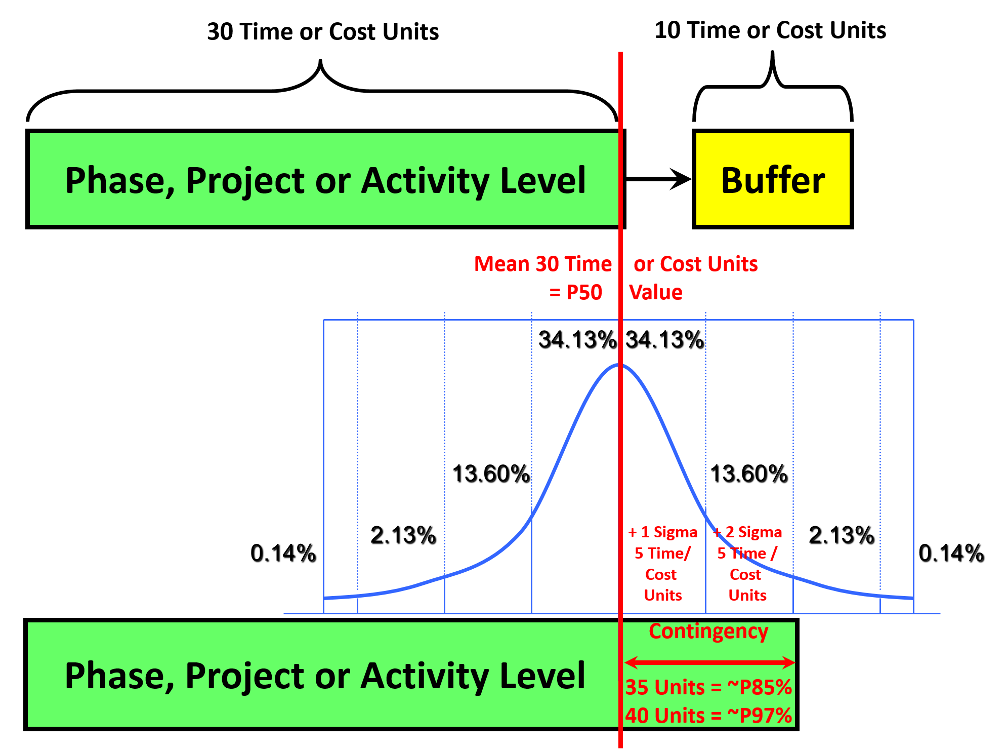
Figure 3 - Buffers and Contingencies

Source: Giammalvo, Paul D (2015) Course Materials. Contributed Under Creative Commons License BY v 4.0

Which approach is “better”?

It all depends on the circumstances but generally speaking, buffers that can be seen tend to get “used” while those which cannot be seen tend to be ignored.

For more on this, see Module 4 - Managing Risk & Opportunity.

07.10.3.7 Prioritizing Risks

Another powerful and useful tool/technique we can use total float for and that is to PRIORITIZE activities based on their total float which determines which activities are more IMPORTANT and the need date, which determines how URGENT they are.

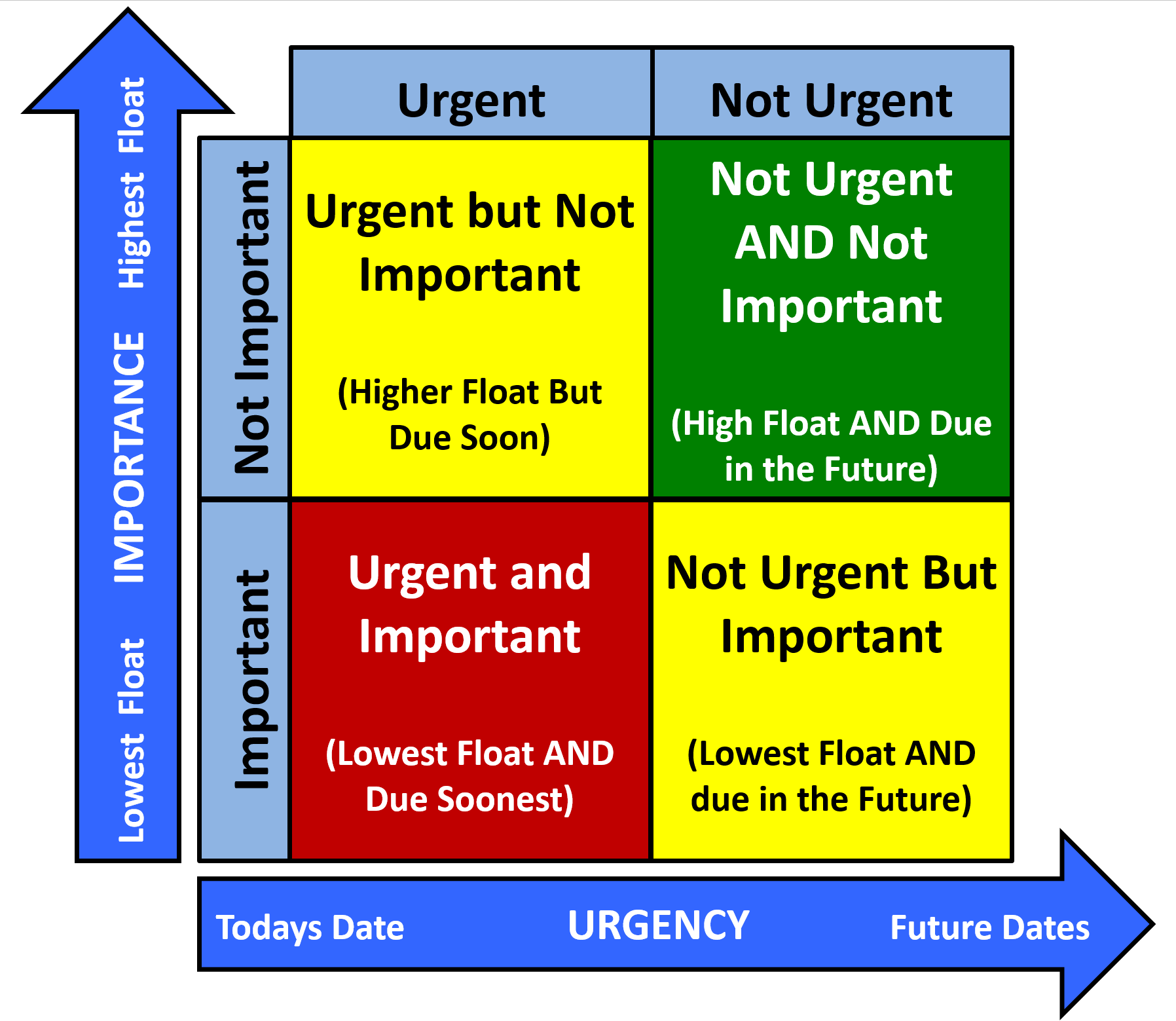
Figure 4 - Importance vs. Urgency Illustrated

Source: Giammalvo, Paul D (2015) Course Materials. Contributed Under Creative Commons License BY v 4.0

A report adopting the above principles can be created by rank ordering (sorting) by Early Start Date (classic waterfall) with a secondary sort by Total Float.  In other words an activity which has negative total float will always be a top priority, as we know negative float is an impossible situation and we must make it go away.

But assuming there is no negative float, then any activity with zero total float and has a scheduled start date of this week is a higher priority than an activity that has zero total float but isn’t due to start for another month.

Obviously, if we discipline ourselves to follow this approach it should give us plenty of time to be able to identify those activities which represent the highest risk to the project and bring them to the attention of the project manager or other key decision makers BEFORE they become a crisis. Thus the priority would be:

• Negative Float whether urgent or not
• Urgent and Important (little or no float and coming up soon)
• Not Urgent but Important (little or no float so it may become negative if not attended to)
• Urgent but Not Important (approaching soon but some float to allow slippage)
• Not Urgent and Not Important. (has float and is off in the future somewhere)

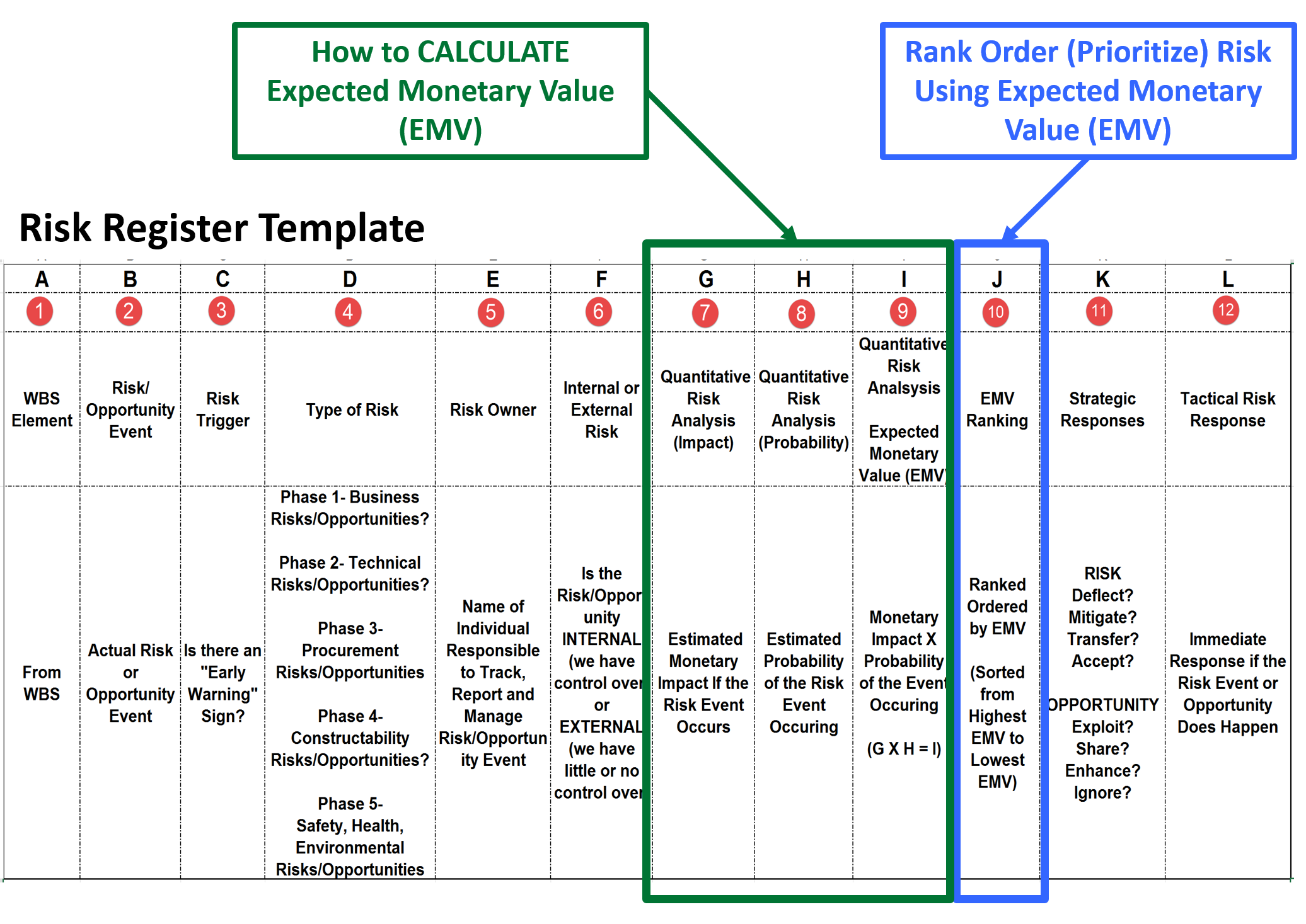
Figure 5 - Calculating Expected Monetary Value (EMV) and Using it to Prioritize Risks

Source: Giammalvo, Paul D (2015) Course Materials. Contributed Under Creative Commons License BY v 4.0

The Risk Register, how to develop it and use it is covered in Module 4 - Managing Risk & Opportunity. However for the purpose of PRIORITIZING RISK events it is done on the basis of Expected Monetary Value which is calculated by taking the probability of the risk even happening, times the impact which for scheduling is monetized by taking the total costs (direct and lost opportunity) for each day delayed and multiplying that times the probability. While this is a very common practice for cost estimators and project control professionals, planners and schedulers rarely seem to do this.

07.10.3.8  Probabilistic Branching / Systems Dynamics

The more likely future of scheduling utilizes systems dynamics software. Unlike the traditional CPM forward pass/backwards pass software which does not allow for LOOPING, using Systems Dynamics software requires that those feedback loops be added. Below is a simplistic graphical illustration:

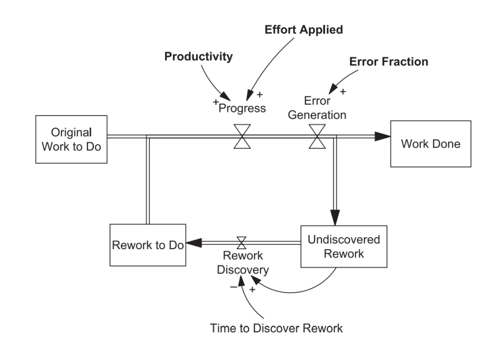
Figure 6 - Probabalistic Branching Illustrated

Source: Lyneis, James and Ford, David (2011)  “System Dynamics applied to Project Management” 

Notice in Figure 6 above that unlike the traditional software packages such as MS Project or Primavera, which use linear algorithm’s to calculate the early and late dates, systems dynamics creates a model of the project which yields probabilities of a project finishing on time and/or within budget.

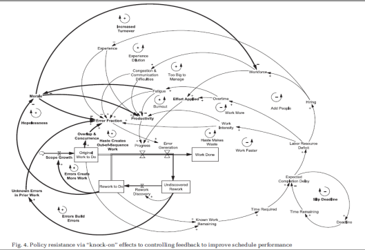
Figure 7 - Showing what a Complete Construction Schedule looks like in Systems Dynamics Software

Source: Lyneis, James and Ford, David (2011)  “System Dynamics applied to Project Managementh” 

For those interested in the evolving application of systems dynamics and systems thinking to project scheduling, here is a link to the paper where the above graphics are explained - “System dynamics applied to project management: a survey, assessment, and directions for future research” 

07.10.4 OUTPUTS

Best Practices Checklist: Conducting a Schedule Risk Analysis:  (Adapted from GAO “Best Practices in Scheduling”)

1. A schedule risk analysis was conducted to determine
2.   -  the likelihood that the project completion date will occur,
3.   -  how much schedule risk contingency is needed to provide an acceptable level of certainty for completion by a specific date,
4.   -  risks most likely to delay the project,
5.   -  how much contingency reserve each risk requires, and
6.   -  the paths or activities that are most likely to delay the project. 
7. The schedule was assessed against best practices before the simulation was conducted. The schedule network clearly identifies work to be done and the relationships between detailed activities and is based on a minimum number of justified date constraints.
8. The schedule risk analysis (SRA) has low, most likely, and high duration data fields.
9. The SRA accounts for correlation in the uncertainty of activity durations.
10. Risks are prioritized by probability and magnitude of impact.
11. The risk register was used in identifying the risk factors potentially driving the schedule before the SRA was conducted.
12. The SRA data and methodology are available and documented.
13. The SRA identifies the activities in the simulation that most often ended up on the critical path, so that near-critical path activities can be closely monitored.
14. The risk inputs have been validated. The ranges are reasonable and based on information gathered from knowledgeable sources, and there is no evidence of bias in the risk data.
15. The baseline schedule includes schedule contingency to account for the occurrence of risks. Schedule contingency is calculated by performing an SRA and comparing the schedule date with that of the simulation result at a desired level of certainty.
16. Schedule contingency is held by the project manager and allocated to contractors, subcontractors, partners, and others as necessary for their scope of work.
17. Contingency is allocated according to the prioritized risk list because the risks that will actually occur and the magnitudes of their effects are not known in advance.
18. The program documents the derivation and amount of contingency set aside by management for risk mitigation and unforeseen problems. An assessment of schedule risk is performed to determine whether the contingency is sufficient.
19. An SRA is performed on the schedule periodically as the schedule is updated to reflect actual progress on activity durations and sequences. A contractor performs an SRA during the formulation of the performance measurement baseline to provide the basis for contractor schedule reserve at the desired confidence level.  

• Updates to the Risk Register
• For advanced practitioners, reference also best practices checklist: conducting a schedule risk analysis see appendix i: an auditor’s key questions and documents page 166-167
• For advanced practitioners reference also best practices checklist: conducting a schedule risk analysis. See appendix iii: standard quantitative measurements for assessing schedule health pages 188 

07.10.5 REFERENCES & TEMPLATES

• GAO “Best Practices in Scheduling"; Best Practice 1
• GAO "Cost Estimating and Assessment guide"; Best Practices for developing and managing capital program costs

07.11 - Module 7-11 - Baselining & Communicating the Schedule

GPCCAR M07-10, Revision 1.01