11.0 - MANAGING PROJECT DATABASES
11.1 - Module 11-1 - Introduction to Managing Project Databases
11.2 - Module 11-2 - Develop the Managing Project Databases Policies and Procedures Manual
11.3 - Module 11-3 - Designing the Project Databases
11.4 - Module 11-4 - Creating the Project Databases
11.5 - MODULE 11-5 - UPDATING AND USING THE PROJECT DATABASE(S)
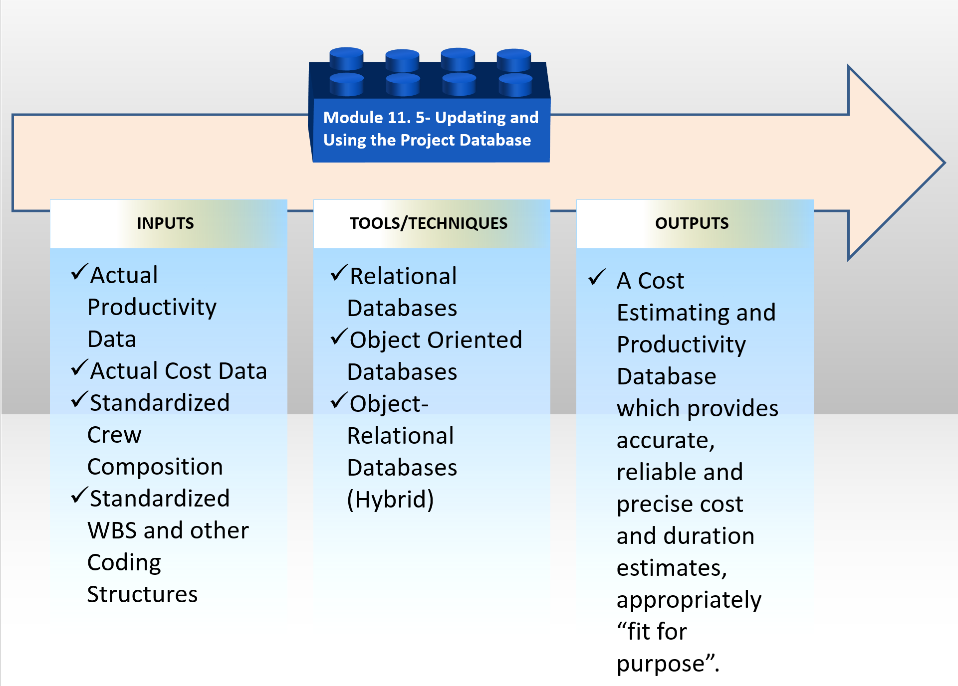
Figure 1 - The Updating and Using the Project Databases Process Map
Source: Guild of Project Controls
11.5.1 - INTRODUCTION
Sources of the Cost and Productivity Databases
For no other reason that R.S Means is probably the oldest (100+ years) and arguably has the largest or most complete databases, we have been using R.S. Means for our examples. (With their permission of course) However, here are many other organizations who offer both general and specialized cost databases:
- SPONS- http://www.franklinandrews.com/publications/spons/
- Hutchins- http://www.franklinandrews.com/publications/hutchins/
- Griffiths- http://www.franklinandrews.com/publications/griffiths/
- Richardson’s- http://www.costdataonline.com/
- Compass- http://www.compassinternational.net/
- Marshal & Swift- https://www.marshallswift.com/faq-43.aspx
From the perspective of practicality, instead of “reinventing the wheel” it is often preferable to purchase one of these “commercial off the shelf” (COTS) databases just for the structure and coding, and then modify the relevant data to fit your area of operations than it is to try to create your own from scratch.
11.5.2 - INPUTS
- Actual (Current) Productivity Data
- Actual (Current) Cost Data
- “Lessons Learned”
11.5.3 - TOOLS & TECHNIQUES
11.5.3.1 What Fields to Update?
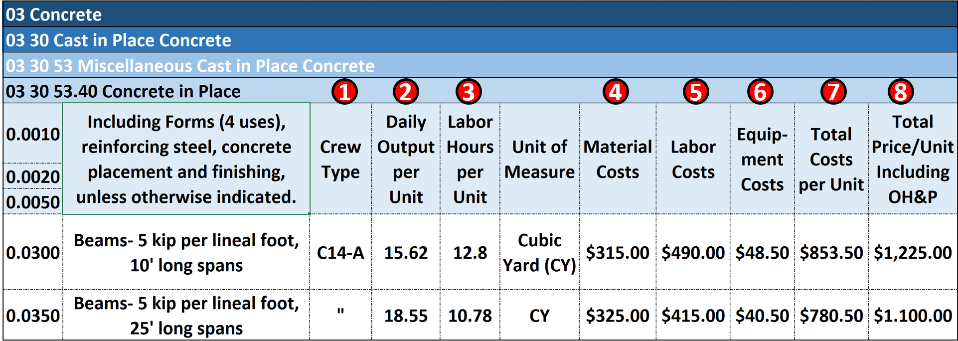
Figure 2 - Modifying the US Park Cost Estimating Database for Use in Scheduling Databases
Source: R.S. Means 2008 Facility Cost Estimating Database
Once you select the commercial off the shelf database OR create your own, you need to populate it with “real” numbers appropriate to your country or region. This means whether you are an owner or contractor, you need to validate the following data fields, however, it is essential that your tracking and reporting, where you capture the input data from the field (Module 9- Managing Progress) is at the same level of detail, which means that your data capture must be using “Activity Based Costing (ABC) and Activity Based Management (ABM) at the level of detail appropriate to your need or application. (Normally for an OWNER it would be Level 3 or Level 4, while for a CONTRACTOR it would be Level 4, Level 5 or even Level 6:
- Crew Type- If the crew TYPE changes or if your crew COMPOSITION changes, then you need to update this field
- Daily Output Per Unit- Based on real time productivity, you need to continuously capture the daily output and using the appropriate Statistical Process Control (SPC) tools/techniques calculate the mean or average value and the probability of any single productivity figure being met or exceeded. See learning curve and statistical process control charts below for more on how to analyse this data prior to inclusion into the database.
- Labor Hours Per Unit- This too will almost certainly exhibit variability and is dependent upon the crew sizes, how well they work together and a host of other variables. As with Output Per Unit in place, the key is for the project controls professional to apply statistical process control chart analysis to the data, throwing out any outliers (those which fall outside of +/- 3 sigma above or below the mean) as well as looking at other patterns which develop in the data which may indicate problems with the process itself.
- Material Costs is self-evident. This can either be validated by simply applying “purchasing power parity”- comparing a “market basket” of materials between any two locations. See more on how to use purchasing power parity below.
- Labor Costs too should be self-evident. These can easily validated by contacting any one of a number of government agencies in nearly all countries who post the various wages for different trades or you can purchase any one of a number of commercial off the shelf databases which contain labor rates for different countries and/or indices to enable you to compare labor rates and productivity between different countries or even different regions within the same country.
- Same with Equipment Costs- With the proliferation of the internet even in the most remote sites, it is possible to find out local equipment rental costs as well as the condition of the equipment and the relative productivity.
- Total Unit Costs are what is important, whether owner or contractor and while there is no single “silver bullet” source, the professional project control practitioner should be able to use his/her network combined with Google searches to locate the current information, analyse it and use it to keep the values in the database updated and current.
- Total Unit Prices, which are the costs marked up to cover contractor’s project overhead, home office overhead, contingency and profit margin become the OWNERS costs. To what the contractor submits to the owner, they too have to add in their project overhead costs, home office overhead, funding costs as well as owners contingency to arrive at the “fair market value”. This again is something that both the contractors and owners project control people have to find from within the organization itself. However “fair market value” can also be found using networking and search engines.
11.5.3.2 “Real” or “Constant” currency using Purchasing Power Parity
The key to consistently being able to produce accurate, reliable and precise cost estimates, which are “fit for purpose” comes from being able to enter accurate numbers into the cost database in the first place, then keep those numbers updated using “real” or “constant” money. Real or constant money is defined to be “Purchasing power of a currency expressed in relation to its purchasing power in a specified year or period. In inflationary times wages are adjusted for the effects of inflation (are 'deflated') by using an index (such as a consumer price index or CPI) to find their worth in constant currency ('in real terms'). See also current dollar [or any other currency].
By far the easiest way to get started is to purchase a database which contains cost and/or productivity data and then update it to reflect local conditions.
However, in today’s world of unstable currencies, professional project controllers are looking to use PURCHASING POWER PARITY as a way to NORMALIZE costs. And there are two approaches.
- One is to use the relative costs of a market basket of goods in one region or time period and then compare the same market basket of goods in another locality and/or point in time. The classic example of this is the Economist’s “Big Mac” Index which started out in 1986 to be a light hearted story, as the index gained credibility it is now used as a reasonably valid indicator of purchasing power parity between any two locations (provided of course they sell Big Macs there).
- Another valid way to measure purchasing power parity which is quickly gaining adherents in today’s world is gold equivalency. The purchasing power of gold has remained remarkably stable over several hundred years. In the 1800’s it took approximately 1 ounce of gold to purchase a good quality man’s suit. And today it costs just about the same- an ounce of gold to purchase a good quality man’s suit.
Without getting into details in this module of how to do this, here are two published articles which have attempted to validate the use of gold equivalency as the basis to project costs into the future: Kumar, Hari S (2012) Exploring Gold as Alternative Currency for Future Cost Estimation in Telecommunication Projects and Asmoro, Trian (2013) Exploring Gold Equivalency for Forecasting Steel Prices on Pipeline Projects.
These papers provide a detailed step by step approach to projecting costs into the future given the unstable global financial situation. Especially for those of you doing long range planning or estimating megaprojects of 3+ years duration, this might prove to be a conservative approach.
11.5.3.3 Construction Cost Indices
One way we can adjust or modify cost data from year to year and/or place to place is by using COST INDICES.
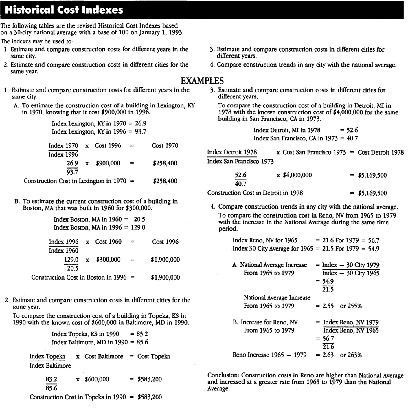
Figure 3 - Showing how to use Cost Indices
Source: Adapted from R.S. Means 2008 Facility Cost Estimating Database
As cost indices are very much location specific, even between one city and another in the same country, if they are not available there is an alternative approach using various forms of “Purchasing Power Parity”. Using Purchasing Power Parity (PPP) you take a “market basket” of goods and services and compare the prices for that same market basket in other cities.
The World Bank and other NGO’s as well as commercial companies publish this data, but by far the easiest and some would argue the most reliable and realistic method is to use the Economist’s “Big Mac Index”. While this started out over 15 years ago as a satire, it quickly gained respect and trust as a relatively reliable, accurate and precise way to compare “real time” costs between any two locations. To use it as an index, we know that in Australia the price of a Big Mac is $2.44 while the price of a Big Mac in America is $3.15.
- Thus to estimate the cost of the same or similar project done in Australia to be done in the USA we would have to increase the cost of the project in the USA by $3.51/$2,44 = 143,9%
We could also take the same approach if the project in Australia was done 5 years ago.
- To do that we would have to find out the price of a Big Mac in Australia and the price of a Big Mac in the USA today and performing the same calculation as above, we could adjust for both TIME and LOCATION.
This can also be done between any two countries.
- Taking the same example as above, we did a project in Australia where the Big Mac costs $2.44 and we want to do the same or similar project in Switzerland, where a Big Mac costs $4.93. To adjust the cost of the same project we did in Australia in Switzerland we would have to increase the price by $4.93/$2.44 or 202%.
It is very important especially for owners to know and understand how to keep their cost databases updated, either based on “real time” bids coming in from their contractors (the most accurate, reliable and precise method or if that information is not accessible then using published indices such as those published by Engineering New Record and if that information is not available then using the Big Mac Index.
There is yet another approach which is gaining some traction in today’s unstable economy and that is known as the Gold Equivalency Method. Because the purchasing power of gold has remained fairly stable for over 200 years (a good quality man’s suit cost what an ounce of gold was back 200 years ago and to buy a good quality man’s suit still costs the same as what an ounce of gold costs today) because it is so stable in terms of purchasing power, it makes an ideal tool to use as an indext.
- To use the gold equivalency method, you take your project costs in Country A and you divide it by the selling price of gold in Country A.
- This will tell you how many ounces of gold your project is worth in Country A.
- Then find out what an ounce of gold sells for in Country B.
- Knowing that you multiply the price of an ounce of gold in Country B x how many ounces of gold your project cost in Country A and you have adjusted for location.
As with previous examples you can also adjust for time as well and if you apply regression analysis you can use and of these indices to project into the future.
Here are two articles, one coming from telecommunications project and another from oil and gas which show you step by step how this is done:
- Sellapan, Hari Kumar, (2012) Exploring Gold as Alternative Currency for Future Cost Estimation in Telecommunication Projects http://pmworldjournal.net/wp-content/uploads/2012/10/PMWJ4-Nov2012-SELL…
- Asmoro, Trian Hendro (2013) Exploring Gold Equivalency for Forecasting Steel Prices on Pipeline Projects http://pmworldjournal.net/wp-content/uploads/2013/05/pmwj10-may2013-asm…
Cost Indexes are published by many organizations including:
- Engineering News Record (ENR) http://enr.construction.com/economics/
- R.S. Means http://rsmeansonline.com/References/CCI/3-Historical%20Cost%20Indexes/1…
- European Union Statistics (EuroStat) http://ec.europa.eu/eurostat/statistics-explained/index.php/Constructio…
- RICS- http://www.rics.org/id/knowledge/glossary/building-costs-around-the-wor…
- EC Harris- http://www.echarris.com/pdf/Intl%20Construction%20Cost%20Report2012FINA…
11.5.3.4 Statistical Process Control Charts
Another important tool/technique which is often over-looked in analyzing cost or productivity data into a cost estimating database is how to identify and eliminate the impact of outliers.
As we know from using Statistical Process Control Charts that any process has normal variation of +/- 3 sigma or 3 standard deviations and any data points which fall outside of +/- 3 sigma are not a normal part of the process but are caused by forces outside of the normal distribution. These are called special or identifiable causes. Looking to our Business Dictionary definition we find that a “special cause” is a Quality control term for that cause of variation which is not an inherent part of a process, but arises out of intermittent, unpredictable, and unstable factors. These extraordinary causes are indicated by data points that fall outside of the limits of a control chart. Also called assignable cause. See also common cause.
Applying this to our cost and productivity data, we need to plot our cost and productivity data, then throw out those readings which fall outside +/- 3 sigma. Failing to do that will result in our data having a high variation. High variation will result in our cost or productivity data being UNRELIABLE as only a few outliers can dramatically skew the values. Thus we need to eliminate them from inclusion in our database.
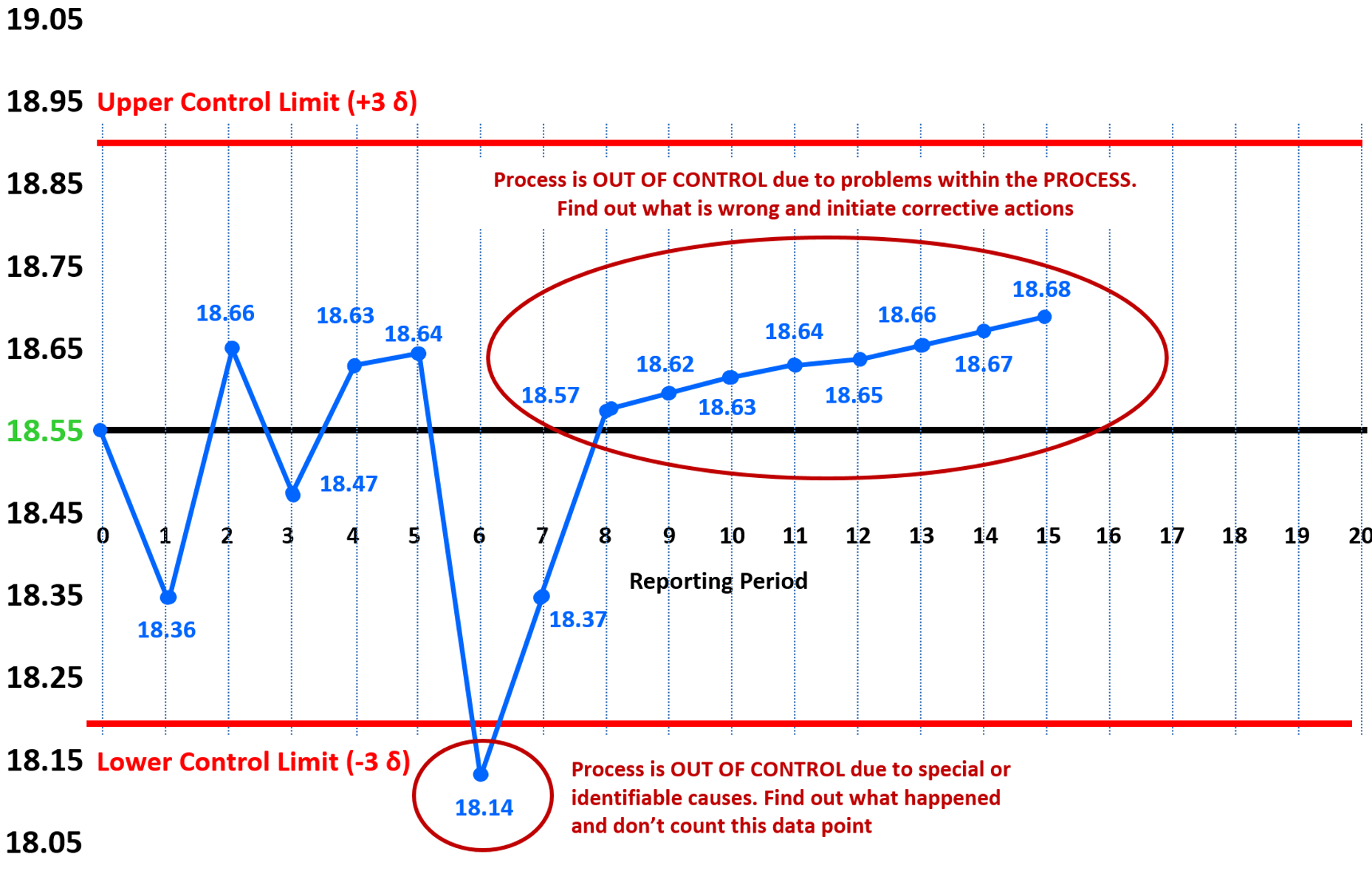
Figure 4 - Using Statistical Process Control Charts
Source: Giammalvo, Paul D (2015) Course Materials Contributed Under Creative Commons License BY v 4.0
Taking the mean productivity from our example above of 18.55 cubic yards per crew day we track the actual productivity per report period and plot it on the appropriate SPC Chart. As we can see while the MEAN or AVERAGE is 18.55 CY per day, the RANGE of “normal” productivity can run from a low of about 18.20 CY per crew day to a high of 18.90 CY per crew day.
We found out that during the reporting period of 5-6, the productivity dropped below the lower control limit. This an indication of a “special” or “identifiable” cause. We spoke with the foreman and he explained that during that entire week, the temperature was above 42 degrees Celsius and it was simply too hot for the crew to be at their maximum productivity. As soon as the heat wave broke, their productivity started to improve. Whenever you have an OUTLIER which falls outside either the upper or lower control limit you do NOT COUNT THAT IN THE DATA BASE. You throw that data point out.
By report period 8, we are back up to near normal productivity but now you start to see a pattern developing. We see the productivity INCREASING every week but whenever you see any patterns developing it means that something MAY be wrong with the process itself. There are many references which show you how to interpret the different patterns you may find but for the purposes of your exam what see shown is known as the “run of 7” (sometimes you also see “run of 6”) What it means is any 6 or 7 consecutive points above the mean, below the mean or ascending or descending, are an indication that the process is out of control due to changes in the process itself. In this case, the project controls team went out to the site and found out the crew was taking shortcuts in the procedure, and while it had a positive impact on the productivity, the changes they made in the process were potentially dangerous and could lead to quality problems with the end product.
Keep in mind that statistical process control (SPC) analysis can be applied to any of the cost or schedule data illustrated above in our ideal database.
The other adjustments we have to make are for PRECISION which is measured by the number of standard deviation from the mean the data falls and for accuracy, which is how close or far away our actual cost or durations are from our original cost or duration estimates. (Adjusted of course for approved change orders).
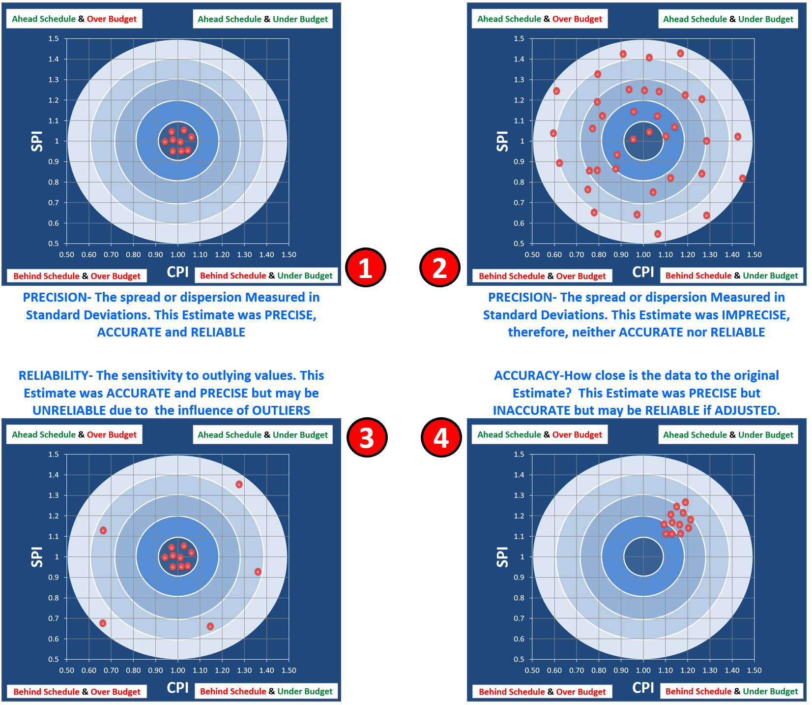
Figure 5 - Precision, Accuracy and Reliability Illustrated
Source: Giammalvo, Paul D (2015) Course Materials. Adapted from Adapted from Rizo, Chris (1999) “Precision, Accuracy and Reliability Illustrated and Contributed Under Creative Commons License BY v 4.0
Like the use of Statistical Process Control Charts this analysis could be applied to any of the productivity or cost data from the database examples above.
Learning Curves
Knowing and understanding how learning curves impact durations is another “tool and technique” that planners / scheduler or cost estimator/project controller can utilise to produce more realistic and achievable schedules and budgets. It can be used for scheduling (durations) as well as for costs.
It is applicable whenever there is a single activity or series of activities (“fragnets”) which repeat on a project. Examples of this are repetitive floor layouts in a hotel or high rise office building, installing pipelines, hanging doors, installing electrical lighting or any other activity or series of activities which repeat.
What learning curves help us do, is knowing how long the first activities are scheduled to take, we can then apply a sound mathematical formula to justify what the subsequent durations are likely to be.
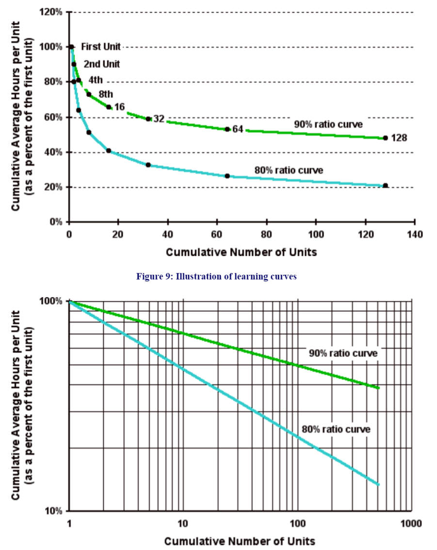
Figure 6 - Learning Curves
Source: Wideman, Max (n.d.) Learning Curve Theory
Whilst many planners / schedulers introduce a slower production rate (say 40 or 50% productivity) for the initial periods or instances for any repetitive operations, a more sound, professionally justifiable approach can also be adopted and applied to the initial periods or instances of the repetitive operations.
The theory behind this is that a learning curve is geometric distribution with the general form “Y = aXb” where:
- Y = cumulative average time per unit or batch.
- a = time taken to produce initial quantity.
- X = the cumulative units of production or, if in batches, the cumulative number of batches.
- b = the learning index or coefficient, which is calculated as: log learning curve percentage ÷ log 2. So b for an 80 per cent curve would be log 0.8 ÷ log 2 = – 0.322.
As we can see from Figure 5 above, we can plot the curve easily using Excel or we can plot it manually using log log paper to generate a straight line. Explained very simply:
- The first time we execute the activity takes us so many minutes, hours or days.
- The second time we execute the activity, it only takes us between 80% to 90% of the time it took us to do it the first time.
- The 4th time we do the activity, it only takes us between 80% to 90% of the time it took us to execute the activity the 2nd time and so on.
- Each time we double the number of times we execute the activity, the time it takes (the number of time periods required) is reduced anywhere between 10% (90% Learning Curve) to 20%. (80% Learning Curve)
As noted, there are two approaches, using units of production or batches and even though the formula is identical. The planner / scheduler can experiment to see which method yields the most accurate results for any specific application. As this tool & technique is applicable to both time and cost, it is an important one for all project control professionals to master, here are recommended supplemental references:
- Bhatti, Ahmad Tariq (2012) Http://Www.Slideshare.Net/Atbhatti/Learning-Curve-15317153
- Brookfield, Bill (2005) Management Accounting – Decision Management Http://Www.Cimaglobal.Com/Documents/Importeddocuments/Fm_April_05_P44-47.Pdf
- Mirsau, Allen (2014) Https://Www.Youtube.Com/Watch?V=Qalpy5inoww
11.5.3.5 Productivity and Cost Adjustment Factors
Other adjustments which need to be taken into consideration when entering new data or updating existing data come to us from published research by the World Academy of Science, Engineering and Technology International Journal of Civil, Environmental, Structural, Construction and Architectural Engineering Vol:8, No:10, 2014 “Labor Productivity in the Construction Industry - Factors Influencing the Spanish Construction Labor Productivity” by G. Robles, A. Stifi, José L. Ponz-Tienda, S. Gentes.
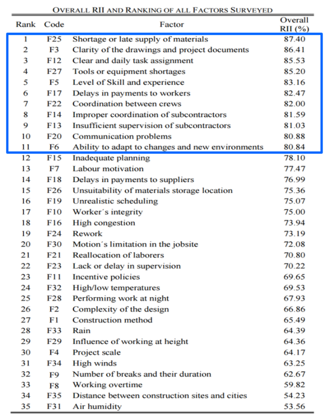
Figure 7 - Productivity Factors
Source: World Academy of Science, Engineering and Technology International Journal of Civil, Environmental, Structural, Construction and Architectural Engineering Vol:8, No:10, 2014 “Labor Productivity in the Construction Industry - Factors Influencing the Spanish Construction Labor Productivity” by G. Robles, A. Stifi, José L. Ponz-Tienda, S. Gentes.
Applying Pareto’s “80:20” rule we need to at least consider whether or not any adjustments to the data can or should be made not only for the top 11 (Pareto’s 80%) but all 35 factors.
Another very important consideration we need to keep in mind and that is the number of days per week scheduled for work. Hours Worked per day/week.
Especially for those owners and contractors working in different countries, the labor laws are not the same and while there is nothing wrong with exceeding the requirements, you may be subject to significant fines if you break these local laws. For example, in the Middle East, you cannot work your field people if the temperature exceed 42 degrees Celsius. Which means you need to change your work calendars during the hot months and/or schedule in two shifts per day rather than three.
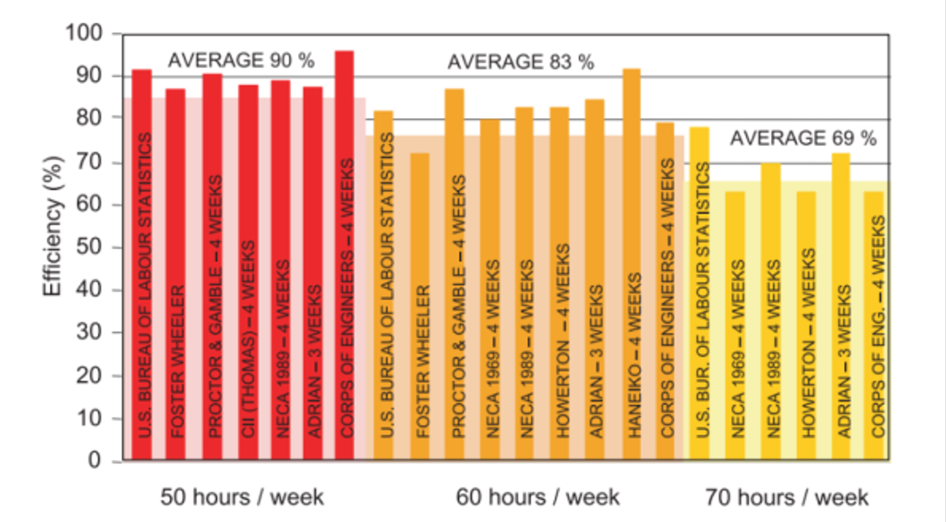
Figure 8 - Revay Report
Source: Source: Revay & Associates(n.d.) The Revay Report
Probably the most complete and comprehensive analysis of the impact overtime has on the project productivity comes to us from the November, 2001 issue of The Revay Report “Calculating Loss of Productivity Due to Overtime Using Published Charts – Fact or Fiction” by Regula Brunies, FPMI, CCC, CQS and Zey Emir, P.Eng, MBA Revay and Associates Limited
Their research concludes that:
- going from a 40 hour work week to a 50 hour workweek we lose on average 10% productivity;
- going to a 60 hour workweek we drop 17% to only 83% from the base productivity and
- going to a 70 hour workweek, we lose 31% productivity,
- dropping down to only 69% of what we can expect working a standard 40 hour workweek.
11.5.4 - OUTPUTS
- A Cost Estimating And Productivity Database Which Provides Accurate, Reliable And Precise Cost And Duration Estimates, Appropriately “Fit For Purpose”.
11.5.5 - REFERENCES & TEMPLATES
- Assignable Vs Random Causes- Https://Surfstat.Anu.Edu.Au/Surfstat-Home/5-1-2.Html • Cost Estimating Databases
- Spons- Http://Www.Franklinandrews.Com/Publications/Spons/
- Hutchins- Http://Www.Franklinandrews.Com/Publications/Hutchins/
- Griffiths- Http://Www.Franklinandrews.Com/Publications/Griffiths/ Richardson’s- Http://Www.Costdataonline.Com/
- Compass- Http://Www.Compassinternational.Net/
- Marshal & Swift- Https://Www.Marshallswift.Com/Faq-43.Aspx
- R.S.Means- Http://Www.Rsmeans.Com/
GPCCAR M11-5, Revision 1.03